44. Sustainable Plans for a Calvo Model#

44.1. Overview#

This is a sequel to this quantecon lecture Time Inconsistency of Ramsey Plans.

That lecture studied a linear-quadratic version of a model that Guillermo Calvo [Calvo, 1978] used to study the time inconsistency of the optimal government plan that emerges when a Stackelberg government (a.k.a. a Ramsey planner) at time $0$ once and for all chooses a sequence $\vec{μ} = {μ_{t}}_{t = 0}^{\infty}$ of gross rates of growth in the supply of money.

A consequence of that choice is a (rational expectations equilibrium) sequence $\vec{θ} = {θ_{t}}_{t = 0}^{\infty}$ of gross rates of increase in the price level that we call inflation rates.

[Calvo, 1978] showed that a Ramsey plan would not emerge from alternative timing protocols and associated supplementary assumptions about what government authorities who set $μ_{t}$ at time $t$ believe how future government authorities who set $μ_{t + j}$ for $j > 0$ will respond to their decisions.

In this lecture, we explore another set of assumptions about what government authorities who set $μ_{t}$ at time $t$ believe how future government authorities who set $μ_{t + j}$ for $j > 0$ will respond to their decisions.

We shall assume that there is sequence of separate policymakers; a time $t$ policymaker chooses only $μ_{t}$ , but now believes that its choice of $μ_{t}$ shapes the representative agent’s beliefs about future rates of money creation and inflation, and through them, future government actions.

This timing protocol and belief structure leads to a model of a credible government policy, also known as a sustainable plan.

In quantecon lecture Time Inconsistency of Ramsey Plans we used ideas from papers by Cagan [Cagan, 1956], Calvo [Calvo, 1978], and Chang [Chang, 1998].

In addition to those ideas, we’ll also use ideas from Abreu [Abreu, 1988], Stokey [Stokey, 1989], [Stokey, 1991], and Chari and Kehoe [Chari and Kehoe, 1990] to study outcomes under our timing protocol.

44.2. Model Components#

We’ll start with a brief review of the setup.

There is no uncertainty.

Let

$p_{t}$ be the log of the price level
$m_{t}$ be the log of nominal money balances
$θ_{t} = p_{t + 1} - p_{t}$ be the net rate of inflation between $t$ and $t + 1$
$μ_{t} = m_{t + 1} - m_{t}$ be the net rate of growth of nominal balances

The demand for real balances is governed by a perfect foresight version of a Cagan [Cagan, 1956] demand function for real balances:

(44.1)#

m_{t} - p_{t} = - α (p_{t + 1} - p_{t}), α > 0

for $t \geq 0$ .

Equation (44.1) asserts that the demand for real balances is inversely related to the public’s expected rate of inflation, which equals the actual rate of inflation because there is no uncertainty here.

(When there is no uncertainty, an assumption of rational expectations that becomes equivalent to perfect foresight).

Subtracting the demand function (44.1) at time $t$ from the demand function at $t + 1$ gives:

μ_{t} - θ_{t} = - α θ_{t + 1} + α θ_{t}

(44.2)#

θ_{t} = \frac{α}{1 + α} θ_{t + 1} + \frac{1}{1 + α} μ_{t}

Because $α > 0$ , $0 < \frac{α}{1 + α} < 1$ .

Definition: For scalar $b_{t}$ , let $L^{2}$ be the space of sequences ${b_{t}}_{t = 0}^{\infty}$ satisfying

\sum_{t = 0}^{\infty} b_{t}^{2} < + \infty

We say that a sequence that belongs to $L^{2}$ is square summable.

When we assume that the sequence $\vec{μ} = {μ_{t}}_{t = 0}^{\infty}$ is square summable and we require that the sequence $\vec{θ} = {θ_{t}}_{t = 0}^{\infty}$ is square summable, the linear difference equation (44.2) can be solved forward to get:

(44.3)#

θ_{t} = \frac{1}{1 + α} \sum_{j = 0}^{\infty} {(\frac{α}{1 + α})}^{j} μ_{t + j}

Insight: In the spirit of Chang [Chang, 1998], equations (44.1) and (44.3) show that $θ_{t}$ intermediates how choices of $μ_{t + j}, j = 0, 1, \dots$ impinge on time $t$ real balances $m_{t} - p_{t} = - α θ_{t}$ .

An equivalence class of continuation money growth sequences ${μ_{t + j}}_{j = 0}^{\infty}$ deliver the same $θ_{t}$ .

That future rates of money creation influence earlier rates of inflation makes timing protocols matter for modeling optimal government policies.

Quantecon lecture Time Inconsistency of Ramsey Plans used this insight to simplify analysis of alternative government policy problems.

44.3. Another Timing Protocol#

The Quantecon lecture Time Inconsistency of Ramsey Plans considered three models of government policy making that differ in

what a policymaker chooses, either a sequence $\vec{μ}$ or just $μ_{t}$ in a single period $t$ .
when a policymaker chooses, either once and for all at time $0$ , or at some time or times $t \geq 0$ .
what a policymaker assumes about how its choice of $μ_{t}$ affects the representative agent’s expectations about inflation rates.

In this lecture, there is a sequence of policymakers, each of whom sets $μ_{t}$ at $t$ only.

To set the stage, recall that in a Markov perfect equilibrium

a time $t$ policymaker cares only about $v_{t}$ and ignores effects that its choice of $μ_{t}$ has on $v_{s}$ at dates $s = 0, 1, \dots, t - 1$ .

In particular, in a Markov perfect equilibrium, there is a sequence indexed by $t = 0, 1, 2, \dots$ of separate policymakers; a time $t$ policymaker chooses $μ_{t}$ only and forecasts that future government decisions are unaffected by its choice.

By way of contrast, in this lecture there is sequence of distinct policymakers; a time $t$ policymaker chooses only $μ_{t}$ , but now believes that its choice of $μ_{t}$ shapes the representative agent’s beliefs about future rates of money creation and inflation, and through them, future government actions.

This timing protocol and belief structure leads to a model of a credible government policy also known as a sustainable plan

The relationship between outcomes under a (Ramsey) timing protocol and the timing protocol and belief structure in this lecture is the subject of a literature on sustainable or credible public policies created by Abreu [Abreu, 1988], [Chari and Kehoe, 1990] [Stokey, 1989], and Stokey [Stokey, 1991].

They discovered conditions under which a Ramsey plan can be rescued from the complaint that it is not credible.

They accomplished this by expanding the description of a plan to include expectations about adverse consequences of deviating from it that can serve to deter deviations.

In this version of our model

the government does not set ${μ_{t}}_{t = 0}^{\infty}$ once and for all at $t = 0$
instead it sets $μ_{t}$ at time $t$
the representative agent’s forecasts of ${μ_{t + j + 1}, θ_{t + j + 1}}_{j = 0}^{\infty}$ respond to whether the government at $t$ confirms or disappoints its forecasts of $μ_{t}$ brought into period $t$ from period $t - 1$ .
the government at each time $t$ understands how the representative agent’s forecasts will respond to its choice of $μ_{t}$ .
at each $t$ , the government chooses $μ_{t}$ to maximize a continuation discounted utility.

44.3.1. Government Decisions#

$\vec{μ}$ is chosen by a sequence of government decision makers, one for each $t \geq 0$ .

The time $t$ decision maker chooses $μ_{t}$ .

We assume the following within-period and between-period timing protocol for each $t \geq 0$ :

at time $t - 1$ , private agents expect that the government will set $μ_{t} = {\tilde{μ}}_{t}$ , and more generally that it will set $μ_{t + j} = {\tilde{μ}}_{t + j}$ for all $j \geq 0$ .
The forecasts ${{\tilde{μ}}_{t + j}}_{j \geq 0}$ determine a $θ_{t} = {\tilde{θ}}_{t}$ and an associated log of real balances $m_{t} - p_{t} = - α {\tilde{θ}}_{t}$ at $t$ .
Given those expectations and an associated $θ_{t} = {\tilde{θ}}_{t}$ , at $t$ a government is free to set $μ_{t} \in R$ .
If the government at $t$ confirms the representative agent’s expectations by setting $μ_{t} = {\tilde{μ}}_{t}$ at time $t$ , private agents expect the continuation government policy ${{\tilde{μ}}_{t + j + 1}}_{j = 0}^{\infty}$ and therefore bring expectation ${\tilde{θ}}_{t + 1}$ into period $t + 1$ .
If the government at $t$ disappoints private agents by setting $μ_{t} \neq {\tilde{μ}}_{t}$ , private agents expect ${μ_{j}^{A}}_{j = 0}^{\infty}$ as the continuation policy for $t + 1$ , i.e., ${μ_{t + j + 1}} = {μ_{j}^{A}}_{j = 0}^{\infty}$ and therefore expect an associated $θ_{0}^{A}$ for $t + 1$ . Here ${\vec{μ}}^{A} = {μ_{j}^{A}}_{j = 0}^{\infty}$ is an alternative government plan to be described below.

44.3.2. Temptation to Deviate from Plan#

The government’s one-period return function $s (θ, μ)$ described in equation (43.10) in quantecon lecture [Calvo, 1978] has the property that for all $θ$

s (θ, 0) \geq s (θ, μ)

This inequality implies that whenever the policy calls for the government to set $μ \neq 0$ , the government could raise its one-period payoff by setting $μ = 0$ .

Disappointing private sector expectations in that way would increase the government’s current payoff but would have adverse consequences for subsequent government payoffs because the private sector would alter its expectations about future settings of $μ$ .

The temporary gain constitutes the government’s temptation to deviate from a plan.

If the government at $t$ is to resist the temptation to raise its current payoff, it is only because it forecasts adverse consequences that its setting of $μ_{t}$ would bring for continuation government payoffs via alterations in the private sector’s expectations.

44.4. Sustainable or Credible Plan#

We call a plan $\vec{μ}$ sustainable or credible if at each $t \geq 0$ the government chooses to confirm private agents’ prior expectation of its setting for $μ_{t}$ .

The government will choose to confirm prior expectations only if the long-term loss from disappointing private sector expectations – coming from the government’s understanding of the way the private sector adjusts its expectations in response to having its prior expectations at $t$ disappointed – outweigh the short-term gain from disappointing those expectations.

The theory of sustainable or credible plans assumes throughout that private sector expectations about what future governments will do are based on the assumption that governments at times $t \geq 0$ always act to maximize the continuation discounted utilities that describe those governments’ purposes.

This aspect of the theory means that credible plans always come in pairs:

a credible (continuation) plan to be followed if the government at $t$ confirms private sector expectations
a credible plan to be followed if the government at $t$ disappoints private sector expectations

That credible plans come in pairs threaten to bring an explosion of plans to keep track of

each credible plan itself consists of two credible plans
therefore, the number of plans underlying one plan is unbounded

But Dilip Abreu showed how to render manageable the number of plans that must be kept track of.

The key is an object called a self-enforcing plan.

We’ll proceed to compute one.

In addition to what’s in Anaconda, this lecture will use the following libraries:

!pip install --upgrade quantecon

We’ll start with some imports:

import numpy as np
from quantecon import LQ
import matplotlib.pyplot as plt
import pandas as pd

44.4.1. Abreu’s Self-Enforcing Plan#

A plan ${\vec{μ}}^{A}$ (here the superscipt $A$ is for Abreu) is said to be self-enforcing if

the consequence of disappointing the representative agent’s expectations at time $j$ is to restart plan ${\vec{μ}}^{A}$ at time $j + 1$
the consequence of restarting the plan is sufficiently adverse that it forever deters all deviations from the plan

More precisely, a government plan ${\vec{μ}}^{A}$ with equilibrium inflation sequence ${\vec{θ}}^{A}$ is self-enforcing if

(44.4)#

\begin{array}{r} \begin{aligned} v_{j}^{A} & = s (θ_{j}^{A}, μ_{j}^{A}) + β v_{j + 1}^{A} \\ \geq s (θ_{j}^{A}, 0) + β v_{0}^{A} \equiv v_{j}^{A, D}, j \geq 0 \end{aligned} \end{array}

(Here it is useful to recall that setting $μ = 0$ is the maximizing choice for the government’s one-period return function)

The first line tells the consequences of confirming the representative agent’s expectations by following the plan, while the second line tells the consequences of disappointing the representative agent’s expectations by deviating from the plan.

A consequence of the inequality stated in the definition is that a self-enforcing plan is credible.

Self-enforcing plans can be used to construct other credible plans, including ones with better values.

Thus, where ${\vec{v}}^{A}$ is the value associated with a self-enforcing plan ${\vec{μ}}^{A}$ , a sufficient condition for another plan $\vec{μ}$ associated with inflation $\vec{θ}$ and value $\vec{v}$ to be credible is that

(44.5)#

\begin{array}{r} \begin{aligned} v_{j} & = s (θ_{j}, μ_{j}) + β v_{j + 1} \\ \geq s (θ_{j}, 0) + β v_{0}^{A} \forall j \geq 0 \end{aligned} \end{array}

For this condition to be satisfied it is necessary and sufficient that

s (θ_{j}, 0) - s (θ_{j}, μ_{j}) < β (v_{j + 1} - v_{0}^{A})

The left side of the above inequality is the government’s gain from deviating from the plan, while the right side is the government’s loss from deviating from the plan.

A government never wants to deviate from a credible plan.

Abreu taught us that key step in constructing a credible plan is first constructing a self-enforcing plan that has a low time $0$ value.

The idea is to use the self-enforcing plan as a continuation plan whenever the government’s choice at time $t$ fails to confirm private agents’ expectation.

We shall use a construction featured in Abreu ([Abreu, 1988]) to construct a self-enforcing plan with low time $0$ value.

44.4.2. Abreu’s Carrot-Stick Plan#

[Abreu, 1988] invented a way to create a self-enforcing plan with a low initial value.

Imitating his idea, we can construct a self-enforcing plan $\vec{μ}$ with a low time $0$ value to the government by insisting that future government decision makers set $μ_{t}$ to a value yielding low one-period utilities to the household for a long time, after which government decisions thereafter yield high one-period utilities.

Low one-period utilities early are a stick
High one-period utilities later are a carrot

Consider a candidate plan ${\vec{μ}}^{A}$ that sets $μ_{t}^{A} = \bar{μ}$ (a high positive number) for $T_{A}$ periods, and then reverts to the Ramsey plan.

Denote this sequence by ${μ_{t}^{A}}_{t = 0}^{\infty}$ .

The sequence of inflation rates implied by this plan, ${θ_{t}^{A}}_{t = 0}^{\infty}$ , can be calculated using:

θ_{t}^{A} = \frac{1}{1 + α} \sum_{j = 0}^{\infty} {(\frac{α}{1 + α})}^{j} μ_{t + j}^{A}

The value of ${θ_{t}^{A}, μ_{t}^{A}}_{t = 0}^{\infty}$ at time $0$ is

v_{0}^{A} = \sum_{t = 0}^{T_{A} - 1} β^{t} s (θ_{t}^{A}, μ_{t}^{A}) + β^{T_{A}} J (θ_{0}^{R})

For an appropriate $T_{A}$ , this plan can be verified to be self-enforcing and therefore credible.

From quantecon lecture Time Inconsistency of Ramsey Plans, we’ll again bring in the Python class ChangLQ that constructs equilibria under timing protocols studied in that lecture.

class ChangLQ:
    """
    Class to solve LQ Chang model
    """
    def __init__(self, β, c, α=1, u0=1, u1=0.5, u2=3, T=1000, θ_n=200):
        # Record parameters
        self.α, self.u0, self.u1, self.u2 = α, u0, u1, u2
        self.β, self.c, self.T, self.θ_n = β, c, T, θ_n

        self.setup_LQ_matrices()
        self.solve_LQ_problem()
        self.compute_policy_functions()
        self.simulate_ramsey_plan()
        self.compute_θ_range()
        self.compute_value_and_policy()

    def setup_LQ_matrices(self):
        # LQ Matrices
        self.R = -np.array([[self.u0, -self.u1 * self.α / 2],
                            [-self.u1 * self.α / 2, 
                             -self.u2 * self.α**2 / 2]])
        self.Q = -np.array([[-self.c / 2]])
        self.A = np.array([[1, 0], [0, (1 + self.α) / self.α]])
        self.B = np.array([[0], [-1 / self.α]])

    def solve_LQ_problem(self):
        # Solve LQ Problem (Subproblem 1)
        lq = LQ(self.Q, self.R, self.A, self.B, beta=self.β)
        self.P, self.F, self.d = lq.stationary_values()

        # Compute g0, g1, and g2 (41.16)
        self.g0, self.g1, self.g2 = [-self.P[0, 0], 
                                     -2 * self.P[1, 0], -self.P[1, 1]]
        
        # Compute b0 and b1 (41.17)
        [[self.b0, self.b1]] = self.F

        # Compute d0 and d1 (41.18)
        self.cl_mat = (self.A - self.B @ self.F)  # Closed loop matrix
        [[self.d0, self.d1]] = self.cl_mat[1:]

        # Solve Subproblem 2
        self.θ_R = -self.P[0, 1] / self.P[1, 1]
        
        # Find the bliss level of θ
        self.θ_B = -self.u1 / (self.u2 * self.α)

    def compute_policy_functions(self):
        # Solve the Markov Perfect Equilibrium
        self.μ_MPE = -self.u1 / ((1 + self.α) / self.α * self.c 
                                 + self.α / (1 + self.α)
                                 * self.u2 + self.α**2 
                                 / (1 + self.α) * self.u2)
        self.θ_MPE = self.μ_MPE
        self.μ_CR = -self.α * self.u1 / (self.u2 * self.α**2 + self.c)
        self.θ_CR = self.μ_CR

        # Calculate value under MPE and CR economy
        self.J_θ = lambda θ_array: - np.array([1, θ_array]) \
                                   @ self.P @ np.array([1, θ_array]).T
        self.V_θ = lambda θ: (self.u0 + self.u1 * (-self.α * θ)
                              - self.u2 / 2 * (-self.α * θ)**2 
                              - self.c / 2 * θ**2) / (1 - self.β)
        
        self.J_MPE = self.V_θ(self.μ_MPE)
        self.J_CR = self.V_θ(self.μ_CR)

    def simulate_ramsey_plan(self):
        # Simulate Ramsey plan for large number of periods
        θ_series = np.vstack((np.ones((1, self.T)), np.zeros((1, self.T))))
        μ_series = np.zeros(self.T)
        J_series = np.zeros(self.T)
        θ_series[1, 0] = self.θ_R
        [μ_series[0]] = -self.F.dot(θ_series[:, 0])
        J_series[0] = self.J_θ(θ_series[1, 0])

        for i in range(1, self.T):
            θ_series[:, i] = self.cl_mat @ θ_series[:, i-1]
            [μ_series[i]] = -self.F @ θ_series[:, i]
            J_series[i] = self.J_θ(θ_series[1, i])

        self.J_series = J_series
        self.μ_series = μ_series
        self.θ_series = θ_series

    def compute_θ_range(self):
        # Find the range of θ in Ramsey plan
        θ_LB = min(min(self.θ_series[1, :]), self.θ_B)
        θ_UB = max(max(self.θ_series[1, :]), self.θ_MPE)
        θ_range = θ_UB - θ_LB
        self.θ_LB = θ_LB - 0.05 * θ_range
        self.θ_UB = θ_UB + 0.05 * θ_range
        self.θ_range = θ_range

    def compute_value_and_policy(self):        
        # Create the θ_space
        self.θ_space = np.linspace(self.θ_LB, self.θ_UB, 200)
        
        # Find value function and policy functions over range of θ
        self.J_space = np.array([self.J_θ(θ) for θ in self.θ_space])
        self.μ_space = -self.F @ np.vstack((np.ones(200), self.θ_space))
        x_prime = self.cl_mat @ np.vstack((np.ones(200), self.θ_space))
        self.θ_prime = x_prime[1, :]
        self.CR_space = np.array([self.V_θ(θ) for θ in self.θ_space])
        
        self.μ_space = self.μ_space[0, :]
        
        # Calculate J_range, J_LB, and J_UB
        self.J_range = np.ptp(self.J_space)
        self.J_LB = np.min(self.J_space) - 0.05 * self.J_range
        self.J_UB = np.max(self.J_space) + 0.05 * self.J_range

Let’s create an instance of ChangLQ with the following parameters:

clq = ChangLQ(β=0.85, c=2)

44.4.3. Example of Self-Enforcing Plan#

The following example implements an Abreu stick-and-carrot plan.

The government sets $μ_{t}^{A} = 0.1$ for $t = 0, 1, \dots, 9$ and then starts the Ramsey plan.

We have computed outcomes for this plan.

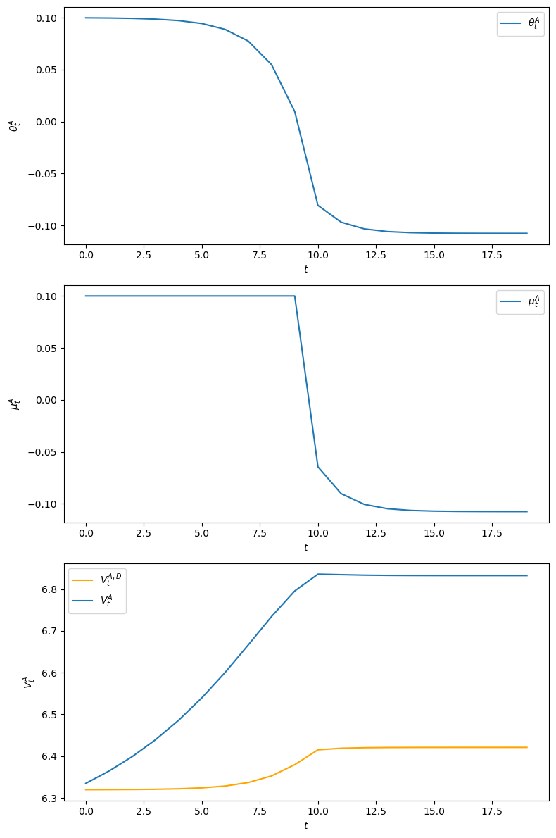
For this plan, we plot the $θ^{A}$ , $μ^{A}$ sequences as well as the implied $v^{A}$ sequence.

Notice that because the government sets money supply growth high for 10 periods, inflation starts high.

Inflation gradually slowly declines because people expect the government to lower the money growth rate after period $10$ .

From the 10th period onwards, the inflation rate $θ_{t}^{A}$ associated with this Abreu plan starts the Ramsey plan from its beginning, i.e., $θ_{t + 10}^{A} = θ_{t}^{R} \forall t \geq 0$ .

_images/82ece591888c6775a546e9721644acdf56e89cd3277d226976892f731c8aedd7.png

To confirm that the plan ${\vec{μ}}^{A}$ is self-enforcing, we plot an object that we call $V_{t}^{A, D}$ , defined in the key inequality in the second line of equation (44.4) above.

$V_{t}^{A, D}$ is the value at $t$ of deviating from the self-enforcing plan ${\vec{μ}}^{A}$ by setting $μ_{t} = 0$ and then restarting the plan at $v_{0}^{A}$ at $t + 1$ :

v_{t}^{A, D} = s (θ_{j}, 0) + β v_{0}^{A}

In the above graph $v_{t}^{A} > v_{t}^{A, D}$ , which confirms that ${\vec{μ}}^{A}$ is a self-enforcing plan.

We can also verify the inequalities required for ${\vec{μ}}^{A}$ to be self-confirming numerically as follows

np.all(clq.V_A[0:20] > clq.V_dev[0:20])

True

Given that plan ${\vec{μ}}^{A}$ is self-enforcing, we can check that the Ramsey plan ${\vec{μ}}^{R}$ is credible by verifying that:

v_{t}^{R} \geq s (θ_{t}^{R}, 0) + β v_{0}^{A}, \forall t \geq 0

def check_ramsey(clq, T=1000):
    # Make sure Ramsey plan is sustainable
    R_dev = np.zeros(T)
    for t in range(T):
        R_dev[t] = (clq.u0 + clq.u1 * (-clq.θ_series[1, t])
                    - clq.u2 / 2 * (-clq.θ_series[1, t])**2) \
                    + clq.β * clq.V_A[0]

    return np.all(clq.J_series > R_dev)

check_ramsey(clq)

True

44.4.4. Recursive Representation of a Sustainable Plan#

We can represent a sustainable plan recursively by taking the continuation value $v_{t}$ as a state variable.

We form the following 3-tuple of functions:

(44.6)#

\begin{array}{r} \begin{aligned} {\hat{μ}}_{t} & = ν_{μ} (v_{t}) \\ θ_{t} & = ν_{θ} (v_{t}) \\ v_{t + 1} & = ν_{v} (v_{t}, μ_{t}) \end{aligned} \end{array}

In addition to these equations, we need an initial value $v_{0}$ to characterize a sustainable plan.

The first equation of (44.6) tells the recommended value of ${\hat{μ}}_{t}$ as a function of the promised value $v_{t}$ .

The second equation of (44.6) tells the inflation rate as a function of $v_{t}$ .

The third equation of (44.6) updates the continuation value in a way that depends on whether the government at $t$ confirms the representative agent’s expectations by setting $μ_{t}$ equal to the recommended value ${\hat{μ}}_{t}$ , or whether it disappoints those expectations.

44.5. Whose Plan is It?#

A credible government plan $\vec{μ}$ plays multiple roles.

It is a sequence of actions chosen by the government.
It is a sequence of the representative agent’s forecasts of government actions.

Thus, $\vec{μ}$ is both a government policy and a collection of the representative agent’s forecasts of government policy.

Does the government choose policy actions or does it simply confirm prior private sector forecasts of those actions?

An argument in favor of the government chooses interpretation comes from noting that the theory of credible plans builds in a theory that the government each period chooses the action that it wants.

An argument in favor of the simply confirm interpretation is gathered from staring at the key inequality (44.5) that defines a credible policy.

We have also computed credible plans for a government or sequence of governments that choose sequentially.

These include

a self-enforcing plan that gives a low initial value $v_{0}$ .
a better plan – possibly one that attains values associated with Ramsey plan – that is not self-enforcing.