18. Growth in Dynamic Linear Economies#

18.3.1. Example 1: Hall (1978)#

First, we set parameters such that consumption follows a random walk. In particular, we set

(In this economy ${\delta }_h$ and ${\theta }_h$ are arbitrary as household capital does not enter the equation for consumption services We set them to values that will become useful in Example 3)

It is worth noting that this choice of parameter values ensures that $\beta ({\gamma }_1+{\delta }_k)=1$.

For simulations of this economy, we choose an initial condition of

# Parameter Matrices
γ_1 = 0.1
ϕ_1 = 1e-5

ϕ_c, ϕ_g, ϕ_i, γ, δ_k, θ_k = (np.array([[1], [0]]),
                              np.array([[0], [1]]),
                              np.array([[1], [-ϕ_1]]),
                              np.array([[γ_1], [0]]),
                              np.array([[.95]]),
                              np.array([[1]]))

β, l_λ, π_h, δ_h, θ_h = (np.array([[1 / 1.05]]),
                         np.array([[0]]),
                         np.array([[1]]),
                         np.array([[.9]]),
                         np.array([[1]]) - np.array([[.9]]))

a22, c2, ub, ud = (np.array([[1,   0,   0],
                             [0, 0.8,   0],
                             [0,   0, 0.5]]),
                   np.array([[0, 0],
                             [1, 0],
                             [0, 1]]),
                   np.array([[30, 0, 0]]),
                   np.array([[5, 1, 0],
                             [0, 0, 0]]))

# Initial condition
x0 = np.array([[5], [150], [1], [0], [0]])

info1 = (a22, c2, ub, ud)
tech1 = (ϕ_c, ϕ_g, ϕ_i, γ, δ_k, θ_k)
pref1 = (β, l_λ, π_h, δ_h, θ_h)

These parameter values are used to define an economy of the DLE class.

econ1 = DLE(info1, tech1, pref1)

We can then simulate the economy for a chosen length of time, from our initial state vector $x_0$

econ1.compute_sequence(x0, ts_length=300)

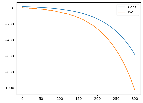
The economy stores the simulated values for each variable. Below we plot consumption and investment

# This is the right panel of Fig 5.7.1 from p.105 of HS2013
plt.plot(econ1.c[0], label='Cons.')
plt.plot(econ1.i[0], label='Inv.')
plt.legend()
plt.show()

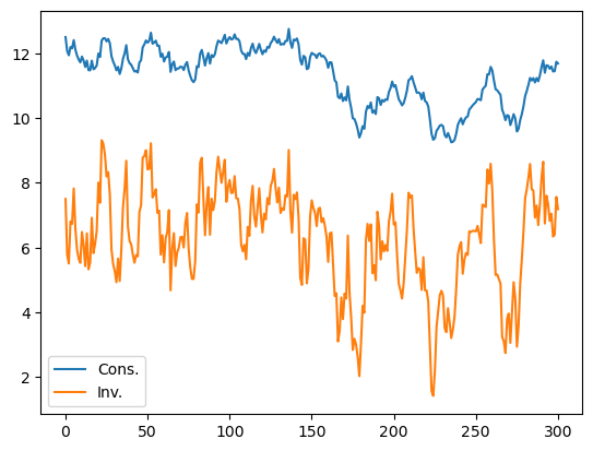
Inspection of the plot shows that the sample paths of consumption and investment drift in ways that suggest that each has or nearly has a random walk or unit root component.

This is confirmed by checking the eigenvalues of $A^o$

econ1.endo, econ1.exo

(array([0.9, 1. ]), array([1. , 0.8, 0.5]))

The endogenous eigenvalue that appears to be unity reflects the random walk character of consumption in Hall’s model.

• Actually, the largest endogenous eigenvalue is very slightly below 1.

• This outcome comes from the small adjustment cost ${\varphi }_1$.

econ1.endo[1]

0.9999999999904767

The fact that the largest endogenous eigenvalue is strictly less than unity in modulus means that it is possible to compute the non-stochastic steady state of consumption, investment and capital.

econ1.compute_steadystate()
np.set_printoptions(precision=3, suppress=True)
print(econ1.css, econ1.iss, econ1.kss)

[[4.999]] [[-0.001]] [[-0.023]]

However, the near-unity endogenous eigenvalue means that these steady state values are of little relevance.

18.3.2. Example 2: Altered Growth Condition#

We generate our next economy by making two alterations to the parameters of Example 1.

• First, we raise ${\varphi }_1$ from 0.00001 to 1.

  • This will lower the endogenous eigenvalue that is close to 1, causing the economy to head more quickly to the vicinity of its non-stochastic steady-state.

• Second, we raise ${\gamma }_1$ from 0.1 to 0.15.

  • This has the effect of raising the optimal steady-state value of capital.

We also start the economy off from an initial condition with a lower capital stock

Therefore, we need to define the following new parameters

γ2 = 0.15
γ22 = np.array([[γ2], [0]])

ϕ_12 = 1
ϕ_i2 = np.array([[1], [-ϕ_12]])

tech2 = (ϕ_c, ϕ_g, ϕ_i2, γ22, δ_k, θ_k)

x02 = np.array([[5], [20], [1], [0], [0]])

Creating the DLE class and then simulating gives the following plot for consumption and investment

econ2 = DLE(info1, tech2, pref1)

econ2.compute_sequence(x02, ts_length=300)

plt.plot(econ2.c[0], label='Cons.')
plt.plot(econ2.i[0], label='Inv.')
plt.legend()
plt.show()

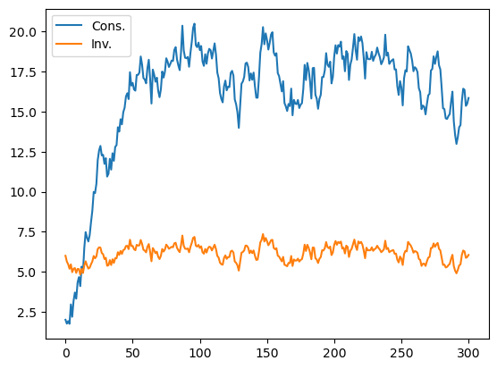
Simulating our new economy shows that consumption grows quickly in the early stages of the sample.

However, it then settles down around the new non-stochastic steady-state level of consumption of 17.5, which we find as follows

econ2.compute_steadystate()
print(econ2.css, econ2.iss, econ2.kss)

[[17.5]] [[6.25]] [[125.]]

The economy converges faster to this level than in Example 1 because the largest endogenous eigenvalue of $A^o$ is now significantly lower than 1.

econ2.endo, econ2.exo

(array([0.9  , 0.952]), array([1. , 0.8, 0.5]))

18.3.3. Example 3: A Jones-Manuelli (1990) Economy#

For our third economy, we choose parameter values with the aim of generating sustained growth in consumption, investment and capital.

To do this, we set parameters so that Jones and Manuelli’s “growth condition” is just satisfied.

In our notation, just satisfying the growth condition is actually equivalent to setting $\beta ({\gamma }_1+{\delta }_k)=1$, the condition that was necessary for consumption to be a random walk in Hall’s model.

Thus, we lower ${\gamma }_1$ back to 0.1.

In our model, this is a necessary but not sufficient condition for growth.

To generate growth we set preference parameters to reflect habit persistence.

In particular, we set $\lambda =-1$, ${\delta }_h=0.9$ and ${\theta }_h=1-{\delta }_h=0.1$.

This makes preferences assume the form

These preferences reflect habit persistence

• the effective “bliss point” $b_t+(1-{\delta }_h)\sum _{j=0}^{\mathrm{\infty }}{\delta }_h^j{c}_{t-j-1}$ now shifts in response to a moving average of past consumption

Since ${\delta }_h$ and ${\theta }_h$ were defined earlier, the only change we need to make from the parameters of Example 1 is to define the new value of $\lambda$.

l_λ2 = np.array([[-1]])
pref2 = (β, l_λ2, π_h, δ_h, θ_h)

econ3 = DLE(info1, tech1, pref2)

We simulate this economy from the original state vector

econ3.compute_sequence(x0, ts_length=300)

# This is the right panel of Fig 5.10.1 from p.110 of HS2013
plt.plot(econ3.c[0], label='Cons.')
plt.plot(econ3.i[0], label='Inv.')
plt.legend()
plt.show()

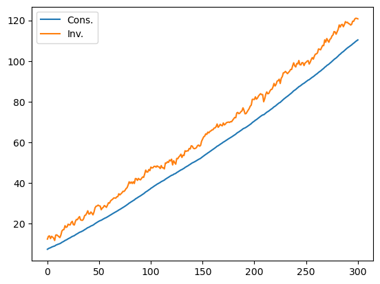
Thus, adding habit persistence to the Hall model of Example 1 is enough to generate sustained growth in our economy.

The eigenvalues of $A^o$ in this new economy are

econ3.endo, econ3.exo

(array([1.+0.j, 1.-0.j]), array([1. , 0.8, 0.5]))

We now have two unit endogenous eigenvalues. One stems from satisfying the growth condition (as in Example 1).

The other unit eigenvalue results from setting $\lambda =-1$.

To show the importance of both of these for generating growth, we consider the following experiments.

18.3.4. Example 3.1: Varying Sensitivity#

Next we raise $\lambda$ to -0.7

l_λ3 = np.array([[-0.7]])
pref3 = (β, l_λ3, π_h, δ_h, θ_h)

econ4 = DLE(info1, tech1, pref3)

econ4.compute_sequence(x0, ts_length=300)

plt.plot(econ4.c[0], label='Cons.')
plt.plot(econ4.i[0], label='Inv.')
plt.legend()
plt.show()

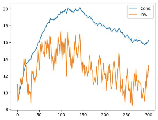
We no longer achieve sustained growth if $\lambda$ is raised from -1 to -0.7.

This is related to the fact that one of the endogenous eigenvalues is now less than 1.

econ4.endo, econ4.exo

(array([0.97, 1.  ]), array([1. , 0.8, 0.5]))

18.3.5. Example 3.2: More Impatience#

Next let’s lower $\beta$ to 0.94

β_2 = np.array([[0.94]])
pref4 = (β_2, l_λ, π_h, δ_h, θ_h)

econ5 = DLE(info1, tech1, pref4)

econ5.compute_sequence(x0, ts_length=300)

plt.plot(econ5.c[0], label='Cons.')
plt.plot(econ5.i[0], label='Inv.')
plt.legend()
plt.show()

Growth also fails if we lower $\beta$, since we now have $\beta ({\gamma }_1+{\delta }_k)<1$.

Consumption and investment explode downwards, as a lower value of $\beta$ causes the representative consumer to front-load consumption.

This explosive path shows up in the second endogenous eigenvalue now being larger than one.

econ5.endo, econ5.exo

(array([0.9  , 1.013]), array([1. , 0.8, 0.5]))