10. How to Pay for a War: Part 2#

10.1. Overview#

This lecture presents another application of Markov jump linear quadratic dynamic programming and constitutes a sequel to an earlier lecture.

We use a method introduced in lecture Markov Jump LQ dynamic programming toimplement suggestions by [Barro, 1999] and [Barro and McCleary, 2003]) for extending his classic 1979 model of tax smoothing.

[Barro, 1979] model is about a government that borrows and lends in order to help it minimize an intertemporal measure of distortions caused by taxes.

Technically, [Barro, 1979] model looks a lot like a consumption-smoothing model.

Our generalizations of [Barro, 1979] will also look like souped-up consumption-smoothing models.

Wanting tractability induced [Barro, 1979] to assume that

the government trades only one-period risk-free debt, and
the one-period risk-free interest rate is constant

In our earlier lecture, we relaxed the second of these assumptions but not the first.

In particular, we used Markov jump linear quadratic dynamic programming to allow the exogenous interest rate to vary over time.

In this lecture, we add a maturity composition decision to the government’s problem by expanding the dimension of the state.

We assume

that the government borrows or saves in the form of risk-free bonds of maturities $1, 2, \dots, H$ .
that interest rates on those bonds are time-varying and in particular are governed by a jointly stationary stochastic process.

In addition to what’s in Anaconda, this lecture deploys the quantecon library:

!pip install --upgrade quantecon

Let’s start with some standard imports:

import quantecon as qe
import numpy as np
import matplotlib.pyplot as plt

10.2. Two example specifications#

We’ll describe two possible specifications

In one, each period the government issues zero-coupon bonds of one- and two-period maturities and redeems them only when they mature – in this version, the maturity structure of government debt at each date is partly inherited from the past.
In the second, the government redesigns the maturity structure of the debt each period.

10.3. One- and Two-period Bonds but No Restructuring#

Let

$T_{t}$ denote tax collections
$β$ be a discount factor
$b_{t, t + 1}$ be time $t + 1$ goods that the government promises to pay at $t$
$b_{t, t + 2}$ betime $t + 2$ goods that the government promises to pay at time $t$
$G_{t}$ be government purchases
$p_{t, t + 1}$ be the number of time $t$ goods received per time $t + 1$ goods promised
$p_{t, t + 2}$ be the number of time $t$ goods received per time $t + 2$ goods promised.

Evidently, $p_{t, t + 1}, p_{t, t + 2}$ are inversely related to appropriate corresponding gross interest rates on government debt.

In the spirit of [Barro, 1979], government expenditures are governed by an exogenous stochastic process.

Given initial conditions $b_{- 2, 0}, b_{- 1, 0}, z_{0}, i_{0}$ , where $i_{0}$ is the initial Markov state, the government chooses a contingency plan for ${b_{t, t + 1}, b_{t, t + 2}, T_{t}}_{t = 0}^{\infty}$ to maximize.

- E_{0} \sum_{t = 0}^{\infty} β^{t} [T_{t}^{2} + c_{1} (b_{t, t + 1} - b_{t, t + 2})^{2}]

subject to the constraints

\begin{aligned} T_{t} & = G_{t} + b_{t - 2, t} + b_{t - 1, t} - p_{t, t + 2} b_{t, t + 2} - p_{t, t + 1} b_{t, t + 1} \\ G_{t} & = U_{g, s_{t}} z_{t} \\ z_{t + 1} & = A_{22, s_{t}} z_{t} + C_{2, s_{t}} w_{t + 1} \\ [\begin{array}{c} p_{t, t + 1} \\ p_{t, t + 2} \\ U_{g, s_{t}} \\ A_{22, s_{t}} \\ C_{2, s_{t}} \end{array}] & \sim functions of Markov state with transition matrix Π \end{aligned}

Here

$w_{t + 1} \sim N (0, I)$ and $Π_{i j}$ is the probability that the Markov state moves from state $i$ to state $j$ in one period
$T_{t}, b_{t, t + 1}, b_{t, t + 2}$ are control variables chosen at time $t$
variables $b_{t - 1, t}, b_{t - 2, t}$ are endogenous state variables inherited from the past at time $t$
$p_{t, t + 1}, p_{t, t + 2}$ are exogenous state variables at time $t$

The parameter $c_{1}$ imposes a penalty on the government’s issuing different quantities of one and two-period debt.

This penalty deters the government from taking large “long-short” positions in debt of different maturities.

An example below will show the penalty in action.

As well as extending the model to allow for a maturity decision for government debt, we can also in principle allow the matrices $U_{g, s_{t}}, A_{22, s_{t}}, C_{2, s_{t}}$ to depend on the Markov state $s_{t}$ .

Below, we will often adopt the convention that for matrices appearing in a linear state space, $A_{t} \equiv A_{s_{t}}, C_{t} \equiv C_{s_{t}}$ and so on, so that dependence on $t$ is always intermediated through the Markov state $s_{t}$ .

10.4. Mapping into an LQ Markov Jump Problem#

First, define

{\hat{b}}_{t} = b_{t - 1, t} + b_{t - 2, t},

which is debt due at time $t$ .

Then define the endogenous part of the state:

{\bar{b}}_{t} = [\begin{matrix} {\hat{b}}_{t} \\ b_{t - 1, t + 1} \end{matrix}]

and the complete state vector

x_{t} = [\begin{matrix} {\bar{b}}_{t} \\ z_{t} \end{matrix}]

and the control vector

u_{t} = [\begin{matrix} b_{t, t + 1} \\ b_{t, t + 2} \end{matrix}]

The endogenous part of state vector follows the law of motion:

[\begin{matrix} {\hat{b}}_{t + 1} \\ b_{t, t + 2} \end{matrix}] = [\begin{matrix} 0 & 1 \\ 0 & 0 \end{matrix}] [\begin{matrix} {\hat{b}}_{t} \\ b_{t - 1, t + 1} \end{matrix}] + [\begin{matrix} 1 & 0 \\ 0 & 1 \end{matrix}] [\begin{matrix} b_{t, t + 1} \\ b_{t, t + 2} \end{matrix}]

{\bar{b}}_{t + 1} = A_{11} {\bar{b}}_{t} + B_{1} u_{t}

Define the following functions of the state

G_{t} = S_{G, t} x_{t}, {\hat{b}}_{t} = S_{1} x_{t}

and

M_{t} = [\begin{matrix} - p_{t, t + 1} & - p_{t, t + 2} \end{matrix}]

where $p_{t, t + 1}$ is the discount on one period loans in the discrete Markov state at time $t$ and $p_{t, t + 2}$ is the discount on two-period loans in the discrete Markov state.

Define

S_{t} = S_{G, t} + S_{1}

Note that in discrete Markov state $i$

T_{t} = M_{t} u_{t} + S_{t} x_{t}

It follows that

T_{t}^{2} = x_{t}^{'} S_{t}^{'} S_{t} x_{t} + u_{t}^{'} M_{t}^{'} M_{t} u_{t} + 2 u_{t}^{'} M_{t}^{'} S_{t} x_{t}

T_{t}^{2} = x_{t}^{'} R_{t} x_{t} + u_{t}^{'} Q_{t} u_{t} + 2 u_{t}^{'} W_{t} x_{t}

where

R_{t} = S_{t}^{'} S_{t}, Q_{t} = M_{t}^{'} M_{t}, W_{t} = M_{t}^{'} S_{t}

Because the payoff function also includes the penalty parameter on issuing debt of different maturities, we have:

T_{t}^{2} + c_{1} (b_{t, t + 1} - b_{t, t + 2})^{2} = x_{t}^{'} R_{t} x_{t} + u_{t}^{'} Q_{t} u_{t} + 2 u_{t}^{'} W_{t} x_{t} + c_{1} u_{t}^{'} Q^{c} u_{t}

where $Q^{c} = [\begin{matrix} 1 & - 1 \\ - 1 & 1 \end{matrix}]$ .

Therefore, the appropriate $Q$ matrix in the Markov jump LQ problem is:

Q_{t}^{c} = Q_{t} + c_{1} Q^{c}

The law of motion of the state in all discrete Markov states $i$ is

x_{t + 1} = A_{t} x_{t} + B u_{t} + C_{t} w_{t + 1}

where

A_{t} = [\begin{matrix} A_{11} & 0 \\ 0 & A_{22, t} \end{matrix}], B = [\begin{matrix} B_{1} \\ 0 \end{matrix}], C_{t} = [\begin{matrix} 0 \\ C_{2, t} \end{matrix}]

Thus, in this problem all the matrices apart from $B$ may depend on the Markov state at time $t$ .

As shown in the previous lecture, when provided with appropriate $A, B, C, R, Q, W$ matrices for each Markov state the LQMarkov class can solve Markov jump LQ problems.

The function below maps the primitive matrices and parameters from the above two-period model into the matrices that the LQMarkov class requires:

def LQ_markov_mapping(A22, C2, Ug, p1, p2, c1=0):

    """
    Function which takes A22, C2, Ug, p_{t, t+1}, p_{t, t+2} and penalty
    parameter c1, and returns the required matrices for the LQMarkov
    model: A, B, C, R, Q, W.
    This version uses the condensed version of the endogenous state.
    """

    # Make sure all matrices can be treated as 2D arrays
    A22 = np.atleast_2d(A22)
    C2 = np.atleast_2d(C2)
    Ug = np.atleast_2d(Ug)
    p1 = np.atleast_2d(p1)
    p2 = np.atleast_2d(p2)

    # Find the number of states (z) and shocks (w)
    nz, nw = C2.shape

    # Create A11, B1, S1, S2, Sg, S matrices
    A11 = np.zeros((2, 2))
    A11[0, 1] = 1

    B1 = np.eye(2)

    S1 = np.hstack((np.eye(1), np.zeros((1, nz+1))))
    Sg = np.hstack((np.zeros((1, 2)), Ug))
    S = S1 + Sg

    # Create M matrix
    M = np.hstack((-p1, -p2))

    # Create A, B, C matrices
    A_T = np.hstack((A11, np.zeros((2, nz))))
    A_B = np.hstack((np.zeros((nz, 2)), A22))
    A = np.vstack((A_T, A_B))

    B = np.vstack((B1, np.zeros((nz, 2))))

    C = np.vstack((np.zeros((2, nw)), C2))

    # Create Q^c matrix
    Qc = np.array([[1, -1], [-1, 1]])

    # Create R, Q, W matrices

    R = S.T @ S
    Q = M.T @ M + c1 * Qc
    W = M.T @ S

    return A, B, C, R, Q, W

With the above function, we can proceed to solve the model in two steps:

Use LQ_markov_mapping to map $U_{g, t}, A_{22, t}, C_{2, t}, p_{t, t + 1}, p_{t, t + 2}$ into the $A, B, C, R, Q, W$ matrices for each of the $n$ Markov states.
Use the LQMarkov class to solve the resulting n-state Markov jump LQ problem.

10.5. Penalty on Different Issues Across Maturities#

To implement a simple example of the two-period model, we assume that $G_{t}$ follows an AR(1) process:

G_{t + 1} = \bar{G} + ρ G_{t} + σ w_{t + 1}

To do this, we set $z_{t} = [\begin{matrix} 1 \\ G_{t} \end{matrix}]$ , and consequently:

\begin{array}{r} A_{22} = [\begin{array}{c} 1 & 0 \\ \bar{G} & ρ \end{array}], C_{2} = [\begin{array}{c} 0 \\ σ \end{array}], U_{g} = [\begin{array}{c} 0 & 1 \end{array}] \end{array}

Therefore, in this example, $A_{22}, C_{2}$ and $U_{g}$ are not time-varying.

We will assume that there are two Markov states, one with a flatter yield curve, and one with a steeper yield curve.

In state 1, prices are:

p_{t, t + 1}^{1} = β, p_{t, t + 2}^{1} = β^{2} - 0.02

and in state 2, prices are:

p_{t, t + 1}^{2} = β, p_{t, t + 2}^{2} = β^{2} + 0.02

We first solve the model with no penalty parameter on different issuance across maturities, i.e. $c_{1} = 0$ .

We specify that the transition matrix for the Markov state is

\begin{array}{r} Π = [\begin{array}{c} 0.9 & 0.1 \\ 0.1 & 0.9 \end{array}] \end{array}

Thus, each Markov state is persistent, and there is an equal chance of moving from one to the other.

# Model parameters
β, Gbar, ρ, σ, c1 = 0.95, 5, 0.8, 1, 0
p1, p2, p3, p4 = β, β**2 - 0.02, β, β**2 + 0.02

# Basic model matrices
A22 = np.array([[1, 0], [Gbar, ρ] ,])
C_2 = np.array([[0], [σ]])
Ug = np.array([[0, 1]])

A1, B1, C1, R1, Q1, W1 = LQ_markov_mapping(A22, C_2, Ug, p1, p2, c1)
A2, B2, C2, R2, Q2, W2 = LQ_markov_mapping(A22, C_2, Ug, p3, p4, c1)

# Small penalties on debt required to implement no-Ponzi scheme
R1[0, 0] = R1[0, 0] + 1e-9
R2[0, 0] = R2[0, 0] + 1e-9

# Construct lists of matrices correspond to each state
As = [A1, A2]
Bs = [B1, B2]
Cs = [C1, C2]
Rs = [R1, R2]
Qs = [Q1, Q2]
Ws = [W1, W2]

Π = np.array([[0.9, 0.1],
              [0.1, 0.9]])

# Construct and solve the model using the LQMarkov class
lqm = qe.LQMarkov(Π, Qs, Rs, As, Bs, Cs=Cs, Ns=Ws, beta=β)
lqm.stationary_values()

# Simulate the model
x0 = np.array([[100, 50, 1, 10]])
x, u, w, t = lqm.compute_sequence(x0, ts_length=300)

# Plot of one and two-period debt issuance
fig, (ax1, ax2) = plt.subplots(1, 2, figsize=(12, 4))
ax1.plot(u[0, :])
ax1.set_title('One-period debt issuance')
ax1.set_xlabel('Time')
ax2.plot(u[1, :])
ax2.set_title('Two-period debt issuance')
ax2.set_xlabel('Time')
plt.show()

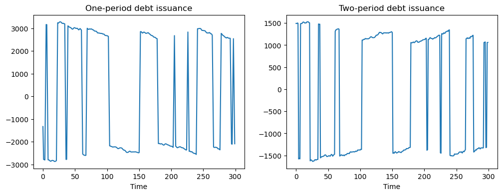
_images/28e7e7dc2a8044f8470188cacd666123a8ab02a064d047c9712063bfcfbfb4c5.png

The above simulations show that when no penalty is imposed on different issuances across maturities, the government has an incentive to take large “long-short” positions in debt of different maturities.

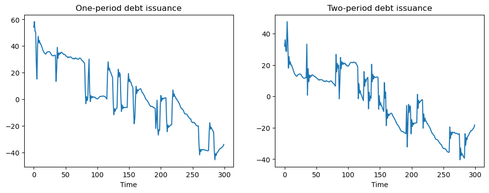
To prevent such outcomes, we set $c_{1} = 0.01$ .

This penalty is big enough to motivate the government to issue positive quantities of both one- and two-period debt:

# Put small penalty on different issuance across maturities
c1 = 0.01

A1, B1, C1, R1, Q1, W1 = LQ_markov_mapping(A22, C_2, Ug, p1, p2, c1)
A2, B2, C2, R2, Q2, W2 = LQ_markov_mapping(A22, C_2, Ug, p3, p4, c1)

# Small penalties on debt required to implement no-Ponzi scheme
R1[0, 0] = R1[0, 0] + 1e-9
R2[0, 0] = R2[0, 0] + 1e-9

# Construct lists of matrices
As = [A1, A2]
Bs = [B1, B2]
Cs = [C1, C2]
Rs = [R1, R2]
Qs = [Q1, Q2]
Ws = [W1, W2]

# Construct and solve the model using the LQMarkov class
lqm2 = qe.LQMarkov(Π, Qs, Rs, As, Bs, Cs=Cs, Ns=Ws, beta=β)
lqm2.stationary_values()

# Simulate the model
x, u, w, t = lqm2.compute_sequence(x0, ts_length=300)

# Plot of one and two-period debt issuance
fig, (ax1, ax2) = plt.subplots(1, 2, figsize=(12, 4))
ax1.plot(u[0, :])
ax1.set_title('One-period debt issuance')
ax1.set_xlabel('Time')
ax2.plot(u[1, :])
ax2.set_title('Two-period debt issuance')
ax2.set_xlabel('Time')
plt.show()

_images/436312df4f117385d67b81b2948b63b1e73e9b6bd284b68344221189d64c92d1.png

10.6. A Model with Restructuring#

We now alter two features of the previous model:

The maximum horizon of government debt is now extended to a general H periods.
The government is able to redesign the maturity structure of debt every period.

We impose a cost on adjusting issuance of each maturity by amending the payoff function to become:

T_{t}^{2} + \sum_{j = 0}^{H - 1} c_{2} (b_{t + j}^{t - 1} - b_{t + j + 1}^{t})^{2}

The government’s budget constraint is now:

T_{t} + \sum_{j = 1}^{H} p_{t, t + j} b_{t + j}^{t} = b_{t}^{t - 1} + \sum_{j = 1}^{H - 1} p_{t, t + j} b_{t + j}^{t - 1} + G_{t}

To map this into the Markov Jump LQ framework, we define state and control variables.

Let:

\begin{array}{r} {\bar{b}}_{t} = [\begin{array}{c} b_{t}^{t - 1} \\ b_{t + 1}^{t - 1} \\ ⋮ \\ b_{t + H - 1}^{t - 1} \end{array}], u_{t} = [\begin{array}{c} b_{t + 1}^{t} \\ b_{t + 2}^{t} \\ ⋮ \\ b_{t + H}^{t} \end{array}] \end{array}

Thus, ${\bar{b}}_{t}$ is the endogenous state (debt issued last period) and $u_{t}$ is the control (debt issued today).

As before, we will also have the exogenous state $z_{t}$ , which determines government spending.

Therefore, the full state is:

\begin{array}{r} x_{t} = [\begin{array}{c} {\bar{b}}_{t} \\ z_{t} \end{array}] \end{array}

We also define a vector $p_{t}$ that contains the time $t$ price of goods in period $t + j$ :

\begin{array}{r} p_{t} = [\begin{array}{c} p_{t, t + 1} \\ p_{t, t + 2} \\ ⋮ \\ p_{t, t + H} \end{array}] \end{array}

Finally, we define three useful matrices $S_{s}, S_{x}, {\tilde{S}}_{x}$ :

\begin{array}{r} [\begin{array}{c} p_{t, t + 1} \\ p_{t, t + 2} \\ ⋮ \\ p_{t, t + H - 1} \end{array}] = S_{s} p_{t} where S_{s} = [\begin{array}{c} 1 & 0 & 0 & \dots & 0 \\ 0 & 1 & 0 & \dots & 0 \\ ⋮ & ⋱ \\ 0 & 0 & \dots & 1 & 0 \end{array}] \end{array}

\begin{array}{r} [\begin{array}{c} b_{t + 1}^{t - 1} \\ b_{t + 2}^{t - 1} \\ ⋮ \\ b_{t + T - 1}^{t - 1} \end{array}] = S_{x} {\bar{b}}_{t} where S_{x} = [\begin{array}{c} 0 & 1 & 0 & \dots & 0 \\ 0 & 0 & 1 & \dots & 0 \\ ⋮ & ⋱ \\ 0 & 0 & \dots & 0 & 1 \end{array}] \end{array}

b_{t}^{t - 1} = {\tilde{S}}_{x} {\bar{b}}_{t} where {\tilde{S}}_{x} = [\begin{matrix} 1 & 0 & 0 & \dots & 0 \end{matrix}]

In terms of dimensions, the first two matrices defined above are $(H - 1) \times H$ .

The last is $1 \times H$

We can now write the government’s budget constraint in matrix notation.

We can rearrange the government budget constraint to become

T_{t} = b_{t}^{t - 1} + \sum_{j = 1}^{H - 1} p_{t + j}^{t} b_{t + j}^{t - 1} + G_{t} - \sum_{j = 1}^{H} p_{t + j}^{t} b_{t + j}^{t}

T_{t} = {\tilde{S}}_{x} {\bar{b}}_{t} + (S_{s} p_{t}) \cdot (S_{x} {\bar{b}}_{t}) + U_{g} z_{t} - p_{t} \cdot u_{t}

To express $T_{t}$ as a function of the full state, let

T_{t} = [\begin{matrix} ({\tilde{S}}_{x} + p_{t}^{'} S_{s}^{'} S_{x}) & U g \end{matrix}] x_{t} - p_{t}^{'} u_{t}

To simplify the notation, let $S_{t} = [\begin{matrix} ({\tilde{S}}_{x} + p_{t}^{'} S_{s}^{'} S_{x}) & U g \end{matrix}]$ .

Then

T_{t} = S_{t} x_{t} - p_{t}^{'} u_{t}

Therefore

T_{t}^{2} = x_{t}^{'} R_{t} x_{t} + u_{t}^{'} Q_{t} u_{t} + 2 u_{t}^{'} W_{t} x_{t}

where

R_{t} = S_{t}^{'} S_{t}, Q_{t} = p_{t} p_{t}^{'}, W_{t} = - p_{t} S_{t}

where to economize on notation we adopt the convention that for the linear state matrices $R_{t} \equiv R_{s_{t}}, Q_{t} \equiv W_{s_{t}}$ and so on.

We’ll use this convention for the linear state matrices $A, B, W$ and so on below.

Because the payoff function also includes the penalty parameter for rescheduling, we have:

T_{t}^{2} + \sum_{j = 0}^{H - 1} c_{2} (b_{t + j}^{t - 1} - b_{t + j + 1}^{t})^{2} = T_{t}^{2} + c_{2} ({\bar{b}}_{t} - u_{t})^{'} ({\bar{b}}_{t} - u_{t})

Because the complete state is $x_{t}$ and not ${\bar{b}}_{t}$ , we rewrite this as:

T_{t}^{2} + c_{2} (S_{c} x_{t} - u_{t})^{'} (S_{c} x_{t} - u_{t})

where $S_{c} = [\begin{matrix} I & 0 \end{matrix}]$

Multiplying this out gives:

T_{t}^{2} + c_{2} x_{t}^{'} S_{c}^{'} S_{c} x_{t} - 2 c_{2} u_{t}^{'} S_{c} x_{t} + c_{2} u_{t}^{'} u_{t}

Therefore, with the cost term, we must amend our $R, Q, W$ matrices as follows:

R_{t}^{c} = R_{t} + c_{2} S_{c}^{'} S_{c}

Q_{t}^{c} = Q_{t} + c_{2} I

W_{t}^{c} = W_{t} - c_{2} S_{c}

To finish mapping into the Markov jump LQ setup, we need to construct the law of motion for the full state.

This is simpler than in the previous setup, as we now have ${\bar{b}}_{t + 1} = u_{t}$ .

Therefore:

\begin{array}{r} x_{t + 1} \equiv [\begin{array}{c} {\bar{b}}_{t + 1} \\ z_{t + 1} \end{array}] = A_{t} x_{t} + B u_{t} + C_{t} w_{t + 1} \end{array}

where

\begin{array}{r} A_{t} = [\begin{array}{c} 0 & 0 \\ 0 & A_{22, t} \end{array}], B = [\begin{array}{c} I \\ 0 \end{array}], C = [\begin{array}{c} 0 \\ C_{2, t} \end{array}] \end{array}

This completes the mapping into a Markov jump LQ problem.

10.7. Restructuring as a Markov Jump Linear Quadratic Control Problem#

We can define a function that maps the primitives of the model with restructuring into the matrices required by the LQMarkov class:

def LQ_markov_mapping_restruct(A22, C2, Ug, T, p_t, c=0):

    """
    Function which takes A22, C2, T, p_t, c and returns the
    required matrices for the LQMarkov model: A, B, C, R, Q, W
    Note, p_t should be a T by 1 matrix
    c is the rescheduling cost (a scalar)
    This version uses the condensed version of the endogenous state
    """

    # Make sure all matrices can be treated as 2D arrays
    A22 = np.atleast_2d(A22)
    C2 = np.atleast_2d(C2)
    Ug = np.atleast_2d(Ug)
    p_t = np.atleast_2d(p_t)

    # Find the number of states (z) and shocks (w)
    nz, nw = C2.shape

    # Create Sx, tSx, Ss, S_t matrices (tSx stands for \tilde S_x)
    Ss = np.hstack((np.eye(T-1), np.zeros((T-1, 1))))
    Sx = np.hstack((np.zeros((T-1, 1)), np.eye(T-1)))
    tSx = np.zeros((1, T))
    tSx[0, 0] = 1

    S_t = np.hstack((tSx + p_t.T @ Ss.T @ Sx, Ug))

    # Create A, B, C matrices
    A_T = np.hstack((np.zeros((T, T)), np.zeros((T, nz))))
    A_B = np.hstack((np.zeros((nz, T)), A22))
    A = np.vstack((A_T, A_B))

    B = np.vstack((np.eye(T), np.zeros((nz, T))))
    C = np.vstack((np.zeros((T, nw)), C2))

    # Create cost matrix Sc
    Sc = np.hstack((np.eye(T), np.zeros((T, nz))))

    # Create R_t, Q_t, W_t matrices

    R_c = S_t.T @ S_t + c * Sc.T @ Sc
    Q_c = p_t @ p_t.T + c * np.eye(T)
    W_c = -p_t @ S_t - c * Sc

    return A, B, C, R_c, Q_c, W_c

10.7.1. Example with Restructuring#

As an example let $H = 3$ .

Assume that there are two Markov states, one with a flatter yield curve, the other with a steeper yield curve.

In state 1, prices are:

p_{t, t + 1}^{1} = 0.9695, p_{t, t + 2}^{1} = 0.902, p_{t, t + 3}^{1} = 0.8369

and in state 2, prices are:

p_{t, t + 1}^{2} = 0.9295, p_{t, t + 2}^{2} = 0.902, p_{t, t + 3}^{2} = 0.8769

We specify the same transition matrix and $G_{t}$ process that we used earlier.

# New model parameters
H = 3
p1 = np.array([[0.9695], [0.902], [0.8369]])
p2 = np.array([[0.9295], [0.902], [0.8769]])
Pi = np.array([[0.9, 0.1], [0.1, 0.9]])

# Put penalty on different issuance across maturities
c2 = 0.5

A1, B1, C1, R1, Q1, W1 = LQ_markov_mapping_restruct(A22, C_2, Ug, H, p1, c2)
A2, B2, C2, R2, Q2, W2 = LQ_markov_mapping_restruct(A22, C_2, Ug, H, p2, c2)

# Small penalties on debt required to implement no-Ponzi scheme
R1[0, 0] = R1[0, 0] + 1e-9
R1[1, 1] = R1[1, 1] + 1e-9
R1[2, 2] = R1[2, 2] + 1e-9
R2[0, 0] = R2[0, 0] + 1e-9
R2[1, 1] = R2[1, 1] + 1e-9
R2[2, 2] = R2[2, 2] + 1e-9

# Construct lists of matrices
As = [A1, A2]
Bs = [B1, B2]
Cs = [C1, C2]
Rs = [R1, R2]
Qs = [Q1, Q2]
Ws = [W1, W2]

# Construct and solve the model using the LQMarkov class
lqm3 = qe.LQMarkov(Π, Qs, Rs, As, Bs, Cs=Cs, Ns=Ws, beta=β)
lqm3.stationary_values()

x0 = np.array([[5000, 5000, 5000, 1, 10]])
x, u, w, t = lqm3.compute_sequence(x0, ts_length=300)

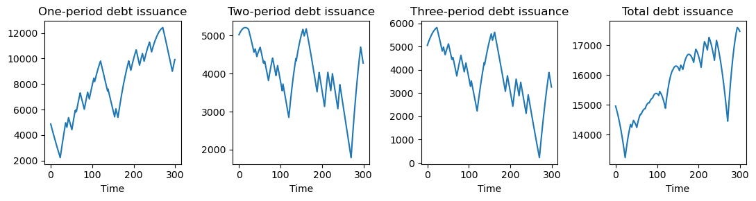
# Plots of different maturities debt issuance

fig, (ax1, ax2, ax3, ax4) = plt.subplots(1, 4, figsize=(11, 3))
ax1.plot(u[0, :])
ax1.set_title('One-period debt issuance')
ax1.set_xlabel('Time')
ax2.plot(u[1, :])
ax2.set_title('Two-period debt issuance')
ax2.set_xlabel('Time')
ax3.plot(u[2, :])
ax3.set_title('Three-period debt issuance')
ax3.set_xlabel('Time')
ax4.plot(u[0, :] + u[1, :] + u[2, :])
ax4.set_title('Total debt issuance')
ax4.set_xlabel('Time')
plt.tight_layout()
plt.show()

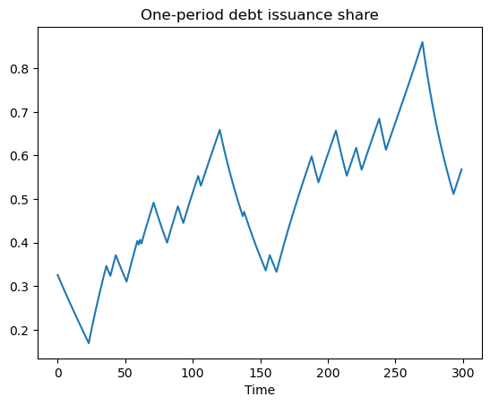
_images/a33a3f512fc5e6a055931429724edae12bdbf00b65db6a2cd2ea0da45a3fa642.png

# Plot share of debt issuance that is short-term

fig, ax = plt.subplots()
ax.plot((u[0, :] / (u[0, :] + u[1, :] + u[2, :])))
ax.set_title('One-period debt issuance share')
ax.set_xlabel('Time')
plt.show()

_images/a98075eaad29ba77e518ddcdc921e4111cd9ff0b2b004838613ee2449756772e.png