22. Rosen Schooling Model#
This lecture is yet another part of a suite of lectures that use the quantecon DLE class to instantiate models within the [Hansen and Sargent, 2013] class of models described in detail in Recursive Models of Dynamic Linear Economies.
In addition to what’s included in Anaconda, this lecture uses the quantecon library
!pip install --upgrade quantecon
We’ll also need the following imports:
import numpy as np
import matplotlib.pyplot as plt
from collections import namedtuple
from quantecon import DLE
22.1. A One-Occupation Model#
Ryoo and Rosen’s (2004) [Ryoo and Rosen, 2004] partial equilibrium model determines
a stock of “Engineers”
a number of new entrants in engineering school,
the wage rate of engineers,
It takes k periods of schooling to become an engineer.
The model consists of the following equations:
a demand curve for engineers:
a time-to-build structure of the education process:
a definition of the discounted present value of each new engineering student:
a supply curve of new students driven by present value
22.2. Mapping into HS2013 Framework#
We represent this model in the [Hansen and Sargent, 2013] framework by
sweeping the time-to-build structure and the demand for engineers into the household technology, and
putting the supply of engineers into the technology for producing goods
22.2.1. Preferences#
where
This specification sets
Below we set things up so that the number of years of education,
22.2.2. Technology#
To capture Ryoo and Rosen’s [Ryoo and Rosen, 2004] supply curve, we use the physical technology:
where
22.2.3. Information#
Because we want
where
Information = namedtuple('Information', ['a22', 'c2','ub','ud'])
Technology = namedtuple('Technology', ['ϕ_c', 'ϕ_g', 'ϕ_i', 'γ', 'δ_k', 'θ_k'])
Preferences = namedtuple('Preferences', ['β', 'l_λ', 'π_h', 'δ_h', 'θ_h'])
22.2.4. Effects of Changes in Education Technology and Demand#
We now study how changing
the number of years of education required to become an engineer and
the slope of the demand curve
affects responses to demand shocks.
To begin, we set
k = 4  # Number of periods of schooling required to become an engineer

β = np.array([[1 / 1.05]])
α_d = np.array([[0.1]])
α_s = 1
ε_1 = 1e-7
λ_1 = np.full((1, k), ε_1)
# Use of ε_1 is trick to aquire detectability, see HS2013 p. 228 footnote 4
l_λ = np.hstack((α_d, λ_1))
π_h = np.array([[0]])

δ_n = np.array([[0.95]])
d1 = np.vstack((δ_n, np.zeros((k - 1, 1))))
d2 = np.hstack((d1, np.eye(k)))
δ_h = np.vstack((d2, np.zeros((1, k + 1))))

θ_h = np.vstack((np.zeros((k, 1)),
                 np.ones((1, 1))))

ψ_1 = 1 / α_s

ϕ_c = np.array([[1], [0]])
ϕ_g = np.array([[0], [-1]])
ϕ_i = np.array([[-1], [ψ_1]])
γ = np.array([[0], [0]])

δ_k = np.array([[0]])
θ_k = np.array([[0]])

ρ_s = 0.8
ρ_d = 0.8

a22 = np.array([[1,   0,   0],
                [0, ρ_s,   0],
                [0,   0, ρ_d]])

c2 = np.array([[0, 0], [10, 0], [0, 10]])
ub = np.array([[30, 0, 1]])
ud = np.array([[10, 1, 0], [0, 0, 0]])

info1 = Information(a22, c2, ub, ud)
tech1 = Technology(ϕ_c, ϕ_g, ϕ_i, γ, δ_k, θ_k)
pref1 = Preferences(β, l_λ, π_h, δ_h, θ_h)

econ1 = DLE(info1, tech1, pref1)
We create three other instances by:
Raising
Raising
Raising
α_d = np.array([[2]])
l_λ = np.hstack((α_d, λ_1))
pref2 = Preferences(β, l_λ, π_h, δ_h, θ_h)
econ2 = DLE(info1, tech1, pref2)

α_d = np.array([[0.1]])

k = 7
λ_1 = np.full((1, k), ε_1)
l_λ = np.hstack((α_d, λ_1))
d1 = np.vstack((δ_n, np.zeros((k - 1, 1))))
d2 = np.hstack((d1, np.eye(k)))
δ_h = np.vstack((d2, np.zeros((1, k+1))))
θ_h = np.vstack((np.zeros((k, 1)),
                 np.ones((1, 1))))

Pref3 = Preferences(β, l_λ, π_h, δ_h, θ_h)
econ3 = DLE(info1, tech1, Pref3)

k = 10
λ_1 = np.full((1, k), ε_1)
l_λ = np.hstack((α_d, λ_1))
d1 = np.vstack((δ_n, np.zeros((k - 1, 1))))
d2 = np.hstack((d1, np.eye(k)))
δ_h = np.vstack((d2, np.zeros((1, k + 1))))
θ_h = np.vstack((np.zeros((k, 1)),
                 np.ones((1, 1))))

pref4 = Preferences(β, l_λ, π_h, δ_h, θ_h)
econ4 = DLE(info1, tech1, pref4)

shock_demand = np.array([[0], [1]])

econ1.irf(ts_length=25, shock=shock_demand)
econ2.irf(ts_length=25, shock=shock_demand)
econ3.irf(ts_length=25, shock=shock_demand)
econ4.irf(ts_length=25, shock=shock_demand)
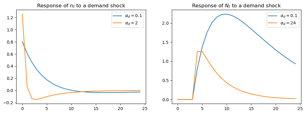
The first figure plots the impulse response of
When
A positive demand shock raises wages, drawing new students into the profession.
However, these new students raise
The higher is
This counteracts the demand shock’s positive effect on wages, reducing the number of new students in subsequent periods.
Consequently, when
fig, (ax1, ax2) = plt.subplots(1, 2, figsize=(12, 4))
ax1.plot(econ1.c_irf,label=r'$\alpha_d = 0.1$')
ax1.plot(econ2.c_irf,label=r'$\alpha_d = 2$')
ax1.legend()
ax1.set_title('Response of $n_t$ to a demand shock')

ax2.plot(econ1.h_irf[:, 0], label=r'$\alpha_d = 0.1$')
ax2.plot(econ2.h_irf[:, 0], label=r'$\alpha_d = 24$')
ax2.legend()
ax2.set_title('Response of $N_t$ to a demand shock')
plt.show()
The next figure plots the impulse response of
fig, (ax1, ax2) = plt.subplots(1, 2, figsize=(12, 4))
ax1.plot(econ1.c_irf, label='$k=4$')
ax1.plot(econ3.c_irf, label='$k=7$')
ax1.plot(econ4.c_irf, label='$k=10$')
ax1.legend()
ax1.set_title('Response of $n_t$ to a demand shock')

ax2.plot(econ1.h_irf[:,0], label='$k=4$')
ax2.plot(econ3.h_irf[:,0], label='$k=7$')
ax2.plot(econ4.h_irf[:,0], label='$k=10$')
ax2.legend()
ax2.set_title('Response of $N_t$ to a demand shock')
plt.show()
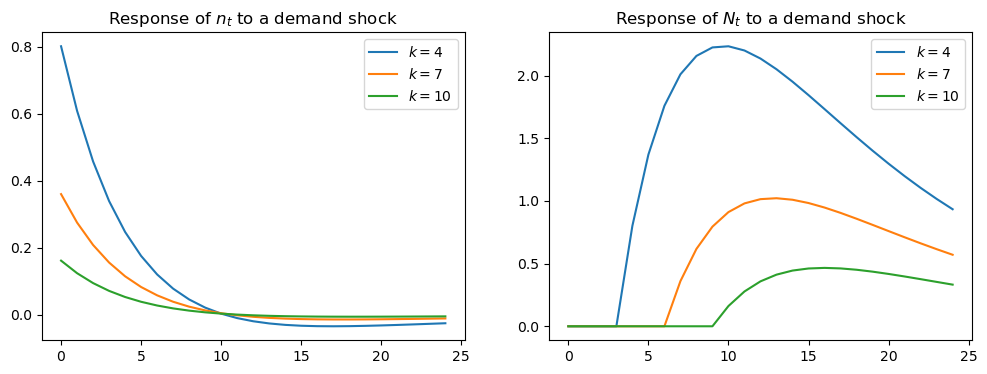
Both panels in the above figure show that raising
Increasing the number of periods of schooling lowers the number of new students in response to a demand shock.
This occurs because with longer required schooling, new students ultimately benefit less from the impact of that shock on wages.