49. Competitive Equilibria of a Model of Chang#

In addition to what’s in Anaconda, this lecture will need the following libraries:

!pip install polytope cvxopt

49.1. Overview#

This lecture describes how Chang [Chang, 1998] analyzed competitive equilibria and a best competitive equilibrium called a Ramsey plan.

He did this by

characterizing a competitive equilibrium recursively in a way also employed in the dynamic Stackelberg problems and Calvo model lectures to pose Stackelberg problems in linear economies, and then
appropriately adapting an argument of Abreu, Pearce, and Stachetti [Abreu et al., 1990] to describe key features of the set of competitive equilibria

Roberto Chang [Chang, 1998] chose a model of Calvo [Calvo, 1978] as a simple structure that conveys ideas that apply more broadly.

A textbook version of Chang’s model appears in chapter 25 of [Ljungqvist and Sargent, 2018].

This lecture and Credible Government Policies in Chang Model can be viewed as more sophisticated and complete treatments of the topics discussed in Ramsey plans, time inconsistency, sustainable plans.

Both this lecture and Credible Government Policies in Chang Model make extensive use of an idea to which we apply the nickname dynamic programming squared.

In dynamic programming squared problems there are typically two interrelated Bellman equations

A Bellman equation for a set of agents or followers with value or value function $v_{a}$ .
A Bellman equation for a principal or Ramsey planner or Stackelberg leader with value or value function $v_{p}$ in which $v_{a}$ appears as an argument.

We encountered problems with this structure in dynamic Stackelberg problems, optimal taxation with state-contingent debt, and other lectures.

We’ll start with some standard imports:

import numpy as np
import polytope
import matplotlib.pyplot as plt

49.1.1. The Setting#

First, we introduce some notation.

For a sequence of scalars $\vec{z} \equiv {z_{t}}_{t = 0}^{\infty}$ , let ${\vec{z}}^{t} = (z_{0}, \dots, z_{t})$ , ${\vec{z}}_{t} = (z_{t}, z_{t + 1}, \dots)$ .

An infinitely lived representative agent and an infinitely lived government exist at dates $t = 0, 1, \dots$ .

The objects in play are

an initial quantity $M_{- 1}$ of nominal money holdings
a sequence of inverse money growth rates $\vec{h}$ and an associated sequence of nominal money holdings $\vec{M}$
a sequence of values of money $\vec{q}$
a sequence of real money holdings $\vec{m}$
a sequence of total tax collections $\vec{x}$
a sequence of per capita rates of consumption $\vec{c}$
a sequence of per capita incomes $\vec{y}$

A benevolent government chooses sequences $(\vec{M}, \vec{h}, \vec{x})$ subject to a sequence of budget constraints and other constraints imposed by competitive equilibrium.

Given tax collection and price of money sequences, a representative household chooses sequences $(\vec{c}, \vec{m})$ of consumption and real balances.

In competitive equilibrium, the price of money sequence $\vec{q}$ clears markets, thereby reconciling decisions of the government and the representative household.

Chang adopts a version of a model that [Calvo, 1978] designed to exhibit time-inconsistency of a Ramsey policy in a simple and transparent setting.

By influencing the representative household’s expectations, government actions at time $t$ affect components of household utilities for periods $s$ before $t$ .

When setting a path for monetary expansion rates, the government takes into account how the household’s anticipations of the government’s future actions affect the household’s current decisions.

The ultimate source of time inconsistency is that a time $0$ Ramsey planner takes these effects into account in designing a plan of government actions for $t \geq 0$ .

49.2. Decisions#

49.2.1. The Household’s Problem#

A representative household faces a nonnegative value of money sequence $\vec{q}$ and sequences $\vec{y}, \vec{x}$ of income and total tax collections, respectively.

Facing vector $\vec{q}$ as a price taker, the representative household chooses nonnegative sequences $\vec{c}, \vec{M}$ of consumption and nominal balances, respectively, to maximize

(49.1)#

\sum_{t = 0}^{\infty} β^{t} [u (c_{t}) + v (q_{t} M_{t})]

subject to

(49.2)#

q_{t} M_{t} \leq y_{t} + q_{t} M_{t - 1} - c_{t} - x_{t}

and

(49.3)#

q_{t} M_{t} \leq \bar{m}

Here $q_{t}$ is the reciprocal of the price level at $t$ , which we can also call the value of money.

Chang [Chang, 1998] assumes that

$u : R_{+} \to R$ is twice continuously differentiable, strictly concave, and strictly increasing;
$v : R_{+} \to R$ is twice continuously differentiable and strictly concave;
$u^{'} (c)_{c \to 0} = lim_{m \to 0} v^{'} (m) = + \infty$ ;
there is a finite level $m = m^{f}$ such that $v^{'} (m^{f}) = 0$

The household carries real balances out of a period equal to $m_{t} = q_{t} M_{t}$ .

Inequality (49.2) is the household’s time $t$ budget constraint.

It tells how real balances $q_{t} M_{t}$ carried out of period $t$ depend on real balances $q_{t} M_{t - 1}$ carried into period $t$ , income, consumption, taxes.

Equation (49.3) imposes an exogenous upper bound $\bar{m}$ on the household’s choice of real balances, where $\bar{m} \geq m^{f}$ .

49.2.2. Government#

The government chooses a sequence of inverse money growth rates with time $t$ component $h_{t} \equiv \frac{M_{t - 1}}{M_{t}} \in Π \equiv [\underset{―}{π}, \overset{―}{π}]$ , where $0 < \underset{―}{π} < 1 < \frac{1}{β} \leq \overset{―}{π}$ .

The government purchases no goods.

It taxes only to acquire paper currency that it will withdraw from circulation (e.g., by burning it).

Let $p_{t}$ be the price level at time $t$ , measured as time $t$ dollars per unit of the consumption good.

Evidently, the value of paper currency meassured in units of the consumption good at time $t$ is

q_{t} = \frac{1}{p_{t}} .

The government faces a sequence of budget constraints with time $t$ component

x_{t} + \frac{M_{t} - M_{t - 1}}{p_{t}} = 0,

where $x_{t}$ is the real value of revenue that the government raises from taxes and $\frac{M_{t} - M_{t - 1}}{p_{t}}$ is the real value of revenue that the government raises by printing new paper currency.

Evidently, this budget constraint can be rewritten as

- x_{t} = q_{t} (M_{t} - M_{t - 1})

which by using the definitions of $m_{t}$ and $h_{t}$ can also be expressed as

(49.4)#

- x_{t} = m_{t} (1 - h_{t})

The restrictions $m_{t} \in [0, \bar{m}]$ and $h_{t} \in Π = [\underset{―}{π}, \overset{―}{π}]$ evidently imply that $x_{t} \in X \equiv [(\underset{―}{π} - 1) \bar{m}, (\overset{―}{π} - 1) \bar{m}]$ .

We define the set $E \equiv [0, \bar{m}] \times Π \times X$ , so that we require that $(m, h, x) \in E$ .

To represent the idea that taxes are distorting, Chang makes the following assumption about outcomes for per capita output:

(49.5)#

y_{t} = f (x_{t}),

where $f : R \to R$ satisfies $f (x) > 0$ , $f (x)$ is twice continuously differentiable, $f^{″} (x) < 0$ , $f^{'} (0) = 0$ , and $f (x) = f (- x)$ for all $x \in R$ , so that subsidies and taxes are equally distorting.

Example parameterizations

In some of our Python code deployed later in this lecture, we’ll assume the following functional forms:

u (c) = \log (c)

v (m) = \frac{1}{500} (m \bar{m} - 0.5 m^{2})^{0.5}

f (x) = 180 - (0.4 x)^{2}

The tax distortion function

Calvo’s and Chang’s purpose is not to model the causes of tax distortions in any detail but simply to summarize the outcome of those distortions via the function $f (x)$ .

A key part of the specification is that tax distortions are increasing in the absolute value of tax revenues.

Ramsey plan: A Ramsey plan is a competitive equilibrium that maximizes (49.1).

Within-period timing of decisions is as follows:

first, the government chooses $h_{t}$ and $x_{t}$ ;
then given $\vec{q}$ and its expectations about future values of $x$ and $y$ ’s, the household chooses $M_{t}$ and therefore $m_{t}$ because $m_{t} = q_{t} M_{t}$ ;
then output $y_{t} = f (x_{t})$ is realized;
finally $c_{t} = y_{t}$

This within-period timing confronts the government with choices framed by how the private sector wants to respond when the government takes time $t$ actions that differ from what the private sector had expected.

This consideration will be important in lecture credible government policies when we study credible government policies.

The model is designed to focus on the intertemporal trade-offs between the welfare benefits of deflation and the welfare costs associated with the high tax collections required to retire money at a rate that delivers deflation.

A benevolent time $0$ government can promote utility generating increases in real balances only by imposing sufficiently large distorting tax collections.

To promote the welfare increasing effects of high real balances, the government wants to induce gradual deflation.

49.2.3. Household’s Problem#

Given $M_{- 1}$ and ${q_{t}}_{t = 0}^{\infty}$ , the household’s problem is

\begin{array}{r} \begin{aligned} L & = max_{\vec{c}, \vec{M}} min_{\vec{λ}, \vec{μ}} \sum_{t = 0}^{\infty} β^{t} {u (c_{t}) + v (M_{t} q_{t}) + λ_{t} [y_{t} - c_{t} - x_{t} + q_{t} M_{t - 1} - q_{t} M_{t}] \\ + μ_{t} [\bar{m} - q_{t} M_{t}]} \end{aligned} \end{array}

First-order conditions with respect to $c_{t}$ and $M_{t}$ , respectively, are

\begin{array}{r} \begin{aligned} u^{'} (c_{t}) & = λ_{t} \\ q_{t} [u^{'} (c_{t}) - v^{'} (M_{t} q_{t})] & \leq β u^{'} (c_{t + 1}) q_{t + 1}, = i f M_{t} q_{t} < \bar{m} \end{aligned} \end{array}

The last equation expresses Karush-Kuhn-Tucker complementary slackness conditions (see here).

These insist that the inequality is an equality at an interior solution for $M_{t}$ .

Using $h_{t} = \frac{M_{t - 1}}{M_{t}}$ and $q_{t} = \frac{m_{t}}{M_{t}}$ in these first-order conditions and rearranging implies

(49.6)#

m_{t} [u^{'} (c_{t}) - v^{'} (m_{t})] \leq β u^{'} (f (x_{t + 1})) m_{t + 1} h_{t + 1}, = if m_{t} < \bar{m}

Define the following key variable

(49.7)#

θ_{t + 1} \equiv u^{'} (f (x_{t + 1})) m_{t + 1} h_{t + 1}

This is real money balances at time $t + 1$ measured in units of marginal utility, which Chang refers to as ‘the marginal utility of real balances’.

From the standpoint of the household at time $t$ , equation (49.7) shows that $θ_{t + 1}$ intermediates the influences of $({\vec{x}}_{t + 1}, {\vec{m}}_{t + 1})$ on the household’s choice of real balances $m_{t}$ .

By “intermediates” we mean that the future paths $({\vec{x}}_{t + 1}, {\vec{m}}_{t + 1})$ influence $m_{t}$ entirely through their effects on the scalar $θ_{t + 1}$ .

The observation that the one dimensional promised marginal utility of real balances $θ_{t + 1}$ functions in this way is an important step in constructing a class of competitive equilibria that have a recursive representation.

A closely related observation pervaded the analysis of Stackelberg plans in lecture dynamic Stackelberg problems.

49.3. Competitive Equilibrium#

Definition:

A government policy is a pair of sequences $(\vec{h}, \vec{x})$ where $h_{t} \in Π \forall t \geq 0$ .
A price system is a nonnegative value of money sequence $\vec{q}$ .
An allocation is a triple of nonnegative sequences $(\vec{c}, \vec{m}, \vec{y})$ .

It is required that time $t$ components $(m_{t}, x_{t}, h_{t}) \in E$ .

Definition:

Given $M_{- 1}$ , a government policy $(\vec{h}, \vec{x})$ , price system $\vec{q}$ , and allocation $(\vec{c}, \vec{m}, \vec{y})$ are said to be a competitive equilibrium if

$m_{t} = q_{t} M_{t}$ and $y_{t} = f (x_{t})$ .
The government budget constraint is satisfied.
Given $\vec{q}, \vec{x}, \vec{y}$ , $(\vec{c}, \vec{m})$ solves the household’s problem.

49.4. Inventory of Objects in Play#

Chang constructs the following objects

A set $Ω$ of initial marginal utilities of money $θ_{0}$
- Let $Ω$ denote the set of initial promised marginal utilities of money $θ_{0}$ associated with competitive equilibria.
- Chang exploits the fact that a competitive equilibrium consists of a first period outcome $(h_{0}, m_{0}, x_{0})$ and a continuation competitive equilibrium with marginal utility of money $θ_{1} \in Ω$ .
Competitive equilibria that have a recursive representation
- A competitive equilibrium with a recursive representation consists of an initial $θ_{0}$ and a four-tuple of functions $(h, m, x, Ψ)$ mapping $θ$ into this period’s $(h, m, x)$ and next period’s $θ$ , respectively.
- A competitive equilibrium can be represented recursively by iterating on
  
  (49.8)# $\begin{array}{r} \begin{aligned} h_{t} & = h (θ_{t}) \\ m_{t} & = m (θ_{t}) \\ x_{t} & = x (θ_{t}) \\ θ_{t + 1} & = Ψ (θ_{t}) \end{aligned} \end{array}$
  
  starting from $θ_{0}$
  
  The range and domain of $Ψ (\cdot)$ are both $Ω$
A recursive representation of a Ramsey plan
- A recursive representation of a Ramsey plan is a recursive competitive equilibrium $θ_{0}, (h, m, x, Ψ)$ that, among all recursive competitive equilibria, maximizes $\sum_{t = 0}^{\infty} β^{t} [u (c_{t}) + v (q_{t} M_{t})]$ .
- The Ramsey planner chooses $θ_{0}, (h, m, x, Ψ)$ from among the set of recursive competitive equilibria at time $0$ .
- Iterations on the function $Ψ$ determine subsequent $θ_{t}$ ’s that summarize the aspects of the continuation competitive equilibria that influence the household’s decisions.
- At time $0$ , the Ramsey planner commits to this implied sequence ${θ_{t}}_{t = 0}^{\infty}$ and therefore to an associated sequence of continuation competitive equilibria.
A characterization of time-inconsistency of a Ramsey plan
- Imagine that after a ‘revolution’ at time $t \geq 1$ , a new Ramsey planner is given the opportunity to ignore history and solve a brand new Ramsey plan.
- This new planner would want to reset the $θ_{t}$ associated with the original Ramsey plan to $θ_{0}$ .
- The incentive to reinitialize $θ_{t}$ associated with this revolution experiment indicates the time-inconsistency of the Ramsey plan.
- By resetting $θ$ to $θ_{0}$ , the new planner avoids the costs at time $t$ that the original Ramsey planner must pay to reap the beneficial effects that the original Ramsey plan for $s \geq t$ had achieved via its influence on the household’s decisions for $s = 0, \dots, t - 1$ .

49.5. Analysis#

A competitive equilibrium is a triple of sequences $(\vec{m}, \vec{x}, \vec{h}) \in E^{\infty}$ that satisfies (49.2), (49.3), and (49.6).

Chang works with a set of competitive equilibria defined as follows.

Definition: $C E = {(\vec{m}, \vec{x}, \vec{h}) \in E^{\infty}$ such that (49.2), (49.3), and (49.6) are satisfied $}$ .

$C E$ is not empty because there exists a competitive equilibrium with $h_{t} = 1$ for all $t \geq 1$ , namely, an equilibrium with a constant money supply and constant price level.

Chang establishes that $C E$ is also compact.

Chang makes the following key observation that combines ideas of Abreu, Pearce, and Stacchetti [Abreu et al., 1990] with insights of Kydland and Prescott [Kydland and Prescott, 1980].

Proposition: The continuation of a competitive equilibrium is a competitive equilibrium.

That is, $(\vec{m}, \vec{x}, \vec{h}) \in C E$ implies that $({\vec{m}}_{t}, {\vec{x}}_{t}, {\vec{h}}_{t}) \in C E \forall t \geq 1$ .

(Lecture dynamic Stackelberg problems also used a version of this insight)

We can now state that a Ramsey problem is to

max_{(\vec{m}, \vec{x}, \vec{h}) \in E^{\infty}} \sum_{t = 0}^{\infty} β^{t} [u (c_{t}) + v (m_{t})]

subject to restrictions (49.2), (49.3), and (49.6).

Evidently, associated with any competitive equilibrium $(m_{0}, x_{0})$ is an implied value of $θ_{0} = u^{'} (f (x_{0})) (m_{0} + x_{0})$ .

To bring out a recursive structure inherent in the Ramsey problem, Chang defines the set

Ω = {θ \in R such that θ = u^{'} (f (x_{0})) (m_{0} + x_{0}) for some (\vec{m}, \vec{x}, \vec{h}) \in C E}

Equation (49.6) inherits from the household’s Euler equation for money holdings the property that the value of $m_{0}$ consistent with the representative household’s choices depends on $({\vec{h}}_{1}, {\vec{m}}_{1})$ .

This dependence is captured in the definition above by making $Ω$ be the set of first period values of $θ_{0}$ satisfying $θ_{0} = u^{'} (f (x_{0})) (m_{0} + x_{0})$ for first period component $(m_{0}, h_{0})$ of competitive equilibrium sequences $(\vec{m}, \vec{x}, \vec{h})$ .

Chang establishes that $Ω$ is a nonempty and compact subset of $R_{+}$ .

Next Chang advances:

Definition: $Γ (θ) = {(\vec{m}, \vec{x}, \vec{h}) \in C E | θ = u^{'} (f (x_{0})) (m_{0} + x_{0})}$ .

Thus, $Γ (θ)$ is the set of competitive equilibrium sequences $(\vec{m}, \vec{x}, \vec{h})$ whose first period components $(m_{0}, h_{0})$ deliver the prescribed value $θ$ for first period marginal utility.

If we knew the sets $Ω, Γ (θ)$ , we could use the following two-step procedure to find at least the value of the Ramsey outcome to the representative household

Find the indirect value function $w (θ)$ defined as

$w (θ) = max_{(\vec{m}, \vec{x}, \vec{h}) \in Γ (θ)} \sum_{t = 0}^{\infty} β^{t} [u (f (x_{t})) + v (m_{t})]$
Compute the value of the Ramsey outcome by solving $max_{θ \in Ω} w (θ)$ .

Thus, Chang states the following

Proposition:

$w (θ)$ satisfies the Bellman equation

(49.9)#

w (θ) = max_{x, m, h, θ^{'}} {u (f (x)) + v (m) + β w (θ^{'})}

where maximization is subject to

(49.10)#

(m, x, h) \in E a n d θ^{'} \in Ω

and

(49.11)#

θ = u^{'} (f (x)) (m + x)

and

(49.12)#

- x = m (1 - h)

and

(49.13)#

m \cdot [u^{'} (f (x)) - v^{'} (m)] \leq β θ^{'}, = i f m < \bar{m}

Before we use this proposition to recover a recursive representation of the Ramsey plan, note that the proposition relies on knowing the set $Ω$ .

To find $Ω$ , Chang uses the insights of Kydland and Prescott [Kydland and Prescott, 1980] together with a method based on the Abreu, Pearce, and Stacchetti [Abreu et al., 1990] iteration to convergence on an operator $B$ that maps continuation values into values.

We want an operator that maps a continuation $θ$ into a current $θ$ .

Chang lets $Q$ be a nonempty, bounded subset of $R$ .

Elements of the set $Q$ are taken to be candidate values for continuation marginal utilities.

Chang defines an operator

B (Q) = θ \in R such that there is (m, x, h, θ^{'}) \in E \times Q

such that (49.11), (49.12), and (49.13) hold.

Thus, $B (Q)$ is the set of first period $θ$ ’s attainable with $(m, x, h) \in E$ and some $θ^{'} \in Q$ .

Proposition:

$Q \subset B (Q)$ implies $B (Q) \subset Ω$ (‘self-generation’).
$Ω = B (Ω)$ (‘factorization’).

The proposition characterizes $Ω$ as the largest fixed point of $B$ .

It is easy to establish that $B (Q)$ is a monotone operator.

This property allows Chang to compute $Ω$ as the limit of iterations on $B$ provided that iterations begin from a sufficiently large initial set.

49.5.1. Some Useful Notation#

Let ${\vec{h}}^{t} = (h_{0}, h_{1}, \dots, h_{t})$ denote a history of inverse money creation rates with time $t$ component $h_{t} \in Π$ .

A government strategy $σ = {σ_{t}}_{t = 0}^{\infty}$ is a $σ_{0} \in Π$ and for $t \geq 1$ a sequence of functions $σ_{t} : Π^{t - 1} \to Π$ .

Chang restricts the government’s choice of strategies to the following space:

C E_{π} = {\vec{h} \in Π^{\infty} : there is some (\vec{m}, \vec{x}) such that (\vec{m}, \vec{x}, \vec{h}) \in C E}

In words, $C E_{π}$ is the set of money growth sequences consistent with the existence of competitive equilibria.

Chang observes that $C E_{π}$ is nonempty and compact.

Definition: $σ$ is said to be admissible if for all $t \geq 1$ and after any history ${\vec{h}}^{t - 1}$ , the continuation ${\vec{h}}_{t}$ implied by $σ$ belongs to $C E_{π}$ .

Admissibility of $σ$ means that anticipated policy choices associated with $σ$ are consistent with the existence of competitive equilibria after each possible subsequent history.

After any history ${\vec{h}}^{t - 1}$ , admissibility restricts the government’s choice in period $t$ to the set

C E_{π}^{0} = {h \in Π : t h e r e i s \vec{h} \in C E_{π} w i t h h = h_{0}}

In words, $C E_{π}^{0}$ is the set of all first period money growth rates $h = h_{0}$ , each of which is consistent with the existence of a sequence of money growth rates $\vec{h}$ starting from $h_{0}$ in the initial period and for which a competitive equilibrium exists.

Remark:

C E_{π}^{0} = {h \in Π : there is (m, θ^{'}) \in [0, \bar{m}] \times Ω such that u^{'} [f ((h - 1) m) - v^{'} (m)] \leq β θ^{'} with equality if m < \bar{m}} .

Definition: An allocation rule is a sequence of functions $\vec{α} = {α_{t}}_{t = 0}^{\infty}$ such that $α_{t} : Π^{t} \to [0, \bar{m}] \times X$ .

Thus, the time $t$ component of $α_{t} (h^{t})$ is a pair of functions $(m_{t} (h^{t}), x_{t} (h^{t}))$ .

Definition: Given an admissible government strategy $σ$ , an allocation rule $α$ is called competitive if given any history ${\vec{h}}^{t - 1}$ and $h_{t} \in C E_{π}^{0}$ , the continuations of $σ$ and $α$ after $({\vec{h}}^{t - 1}, h_{t})$ induce a competitive equilibrium sequence.

49.5.2. Another Operator#

At this point it is convenient to introduce another operator that can be used to compute a Ramsey plan.

For computing a Ramsey plan, this operator is wasteful because it works with a state vector that is bigger than necessary.

We introduce this operator because it helps to prepare the way for Chang’s operator called $\tilde{D} (Z)$ that we shall describe in lecture credible government policies.

It is also useful because a fixed point of the operator to be defined here provides a good guess for an initial set from which to initiate iterations on Chang’s set-to-set operator $\tilde{D} (Z)$ to be described in lecture credible government policies.

Let $S$ be the set of all pairs $(w, θ)$ of competitive equilibrium values and associated initial marginal utilities.

Let $W$ be a bounded set of values in $R$ .

Let $Z$ be a nonempty subset of $W \times Ω$ .

Think of using pairs $(w^{'}, θ^{'})$ drawn from $Z$ as candidate continuation value, $θ$ pairs.

Define the operator

D (Z) = {(w, θ) : t h e r e i s h \in C E_{π}^{0}

and a four-tuple (m (h), x (h), w^{'} (h), θ^{'} (h)) \in [0, \bar{m}] \times X \times Z

such that

(49.14)#

w = u (f (x (h))) + v (m (h)) + β w^{'} (h)

(49.15)#

θ = u^{'} (f (x (h))) (m (h) + x (h))

(49.16)#

x (h) = m (h) (h - 1)

(49.17)#

m (h) (u^{'} (f (x (h))) - v^{'} (m (h))) \leq β θ^{'} (h)

with equality if m (h) < \bar{m}}

It is possible to establish.

Proposition:

If $Z \subset D (Z)$ , then $D (Z) \subset S$ (‘self-generation’).
$S = D (S)$ (‘factorization’).

Proposition:

Monotonicity of $D$ : $Z \subset Z^{'}$ implies $D (Z) \subset D (Z^{'})$ .
$Z$ compact implies that $D (Z)$ is compact.

It can be shown that $S$ is compact and that therefore there exists a $(w, θ)$ pair within this set that attains the highest possible value $w$ .

This $(w, θ)$ pair i associated with a Ramsey plan.

Further, we can compute $S$ by iterating to convergence on $D$ provided that one begins with a sufficiently large initial set $S_{0}$ .

As a very useful by-product, the algorithm that finds the largest fixed point $S = D (S)$ also produces the Ramsey plan, its value $w$ , and the associated competitive equilibrium.

49.6. Calculating all Promise-Value Pairs in CE#

Above we have defined the $D (Z)$ operator as:

D (Z) = {(w, θ) : \exists h \in C E_{π}^{0} and (m (h), x (h), w^{'} (h), θ^{'} (h)) \in [0, \bar{m}] \times X \times Z

such that

w = u (f (x (h))) + v (m (h)) + β w^{'} (h)

θ = u^{'} (f (x (h))) (m (h) + x (h))

x (h) = m (h) (h - 1)

m (h) (u^{'} (f (x (h))) - v^{'} (m (h))) \leq β θ^{'} (h) (with equality if m (h) < \bar{m})}

We noted that the set $S$ can be found by iterating to convergence on $D$ , provided that we start with a sufficiently large initial set $S_{0}$ .

Our implementation builds on ideas in this notebook.

To find $S$ we use a numerical algorithm called the outer hyperplane approximation algorithm.

It was invented by Judd, Yeltekin, Conklin [Judd et al., 2003].

This algorithm constructs the smallest convex set that contains the fixed point of the $D (S)$ operator.

Given that we are finding the smallest convex set that contains $S$ , we can represent it on a computer as the intersection of a finite number of half-spaces.

Let $H$ be a set of subgradients, and $C$ be a set of hyperplane levels.

We approximate $S$ by:

\tilde{S} = {(w, θ) | H \cdot (w, θ) \leq C}

A key feature of this algorithm is that we discretize the action space, i.e., we create a grid of possible values for $m$ and $h$ (note that $x$ is implied by $m$ and $h$ ). This discretization simplifies computation of $\tilde{S}$ by allowing us to find it by solving a sequence of linear programs.

The outer hyperplane approximation algorithm proceeds as follows:

Initialize subgradients, $H$ , and hyperplane levels, $C_{0}$ .
Given a set of subgradients, $H$ , and hyperplane levels, $C_{t}$ , for each subgradient $h_{i} \in H$ :
- Solve a linear program (described below) for each action in the action space.
- Find the maximum and update the corresponding hyperplane level, $C_{i, t + 1}$ .
If $| C_{t + 1} - C_{t} | > ε$ , return to 2.

Step 1 simply creates a large initial set $S_{0}$ .

Given some set $S_{t}$ , Step 2 then constructs the set $S_{t + 1} = D (S_{t})$ . The linear program in Step 2 is designed to construct a set $S_{t + 1}$ that is as large as possible while satisfying the constraints of the $D (S)$ operator.

To do this, for each subgradient $h_{i}$ , and for each point in the action space $(m_{j}, h_{j})$ , we solve the following problem:

max_{[w^{'}, θ^{'}]} h_{i} \cdot (w, θ)

subject to

H \cdot (w^{'}, θ^{'}) \leq C_{t}

w = u (f (x_{j})) + v (m_{j}) + β w^{'}

θ = u^{'} (f (x_{j})) (m_{j} + x_{j})

x_{j} = m_{j} (h_{j} - 1)

m_{j} (u^{'} (f (x_{j})) - v^{'} (m_{j})) \leq β θ^{'} (= if m_{j} < \bar{m})

This problem maximizes the hyperplane level for a given set of actions.

The second part of Step 2 then finds the maximum possible hyperplane level across the action space.

The algorithm constructs a sequence of progressively smaller sets $S_{t + 1} \subset S_{t} \subset S_{t - 1} \dots \subset S_{0}$ .

Step 3 ends the algorithm when the difference between these sets is small enough.

We have created a Python class that solves the model assuming the following functional forms:

u (c) = \log (c)

v (m) = \frac{1}{500} (m \bar{m} - 0.5 m^{2})^{0.5}

f (x) = 180 - (0.4 x)^{2}

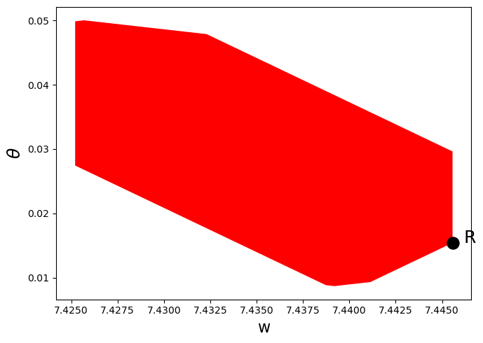
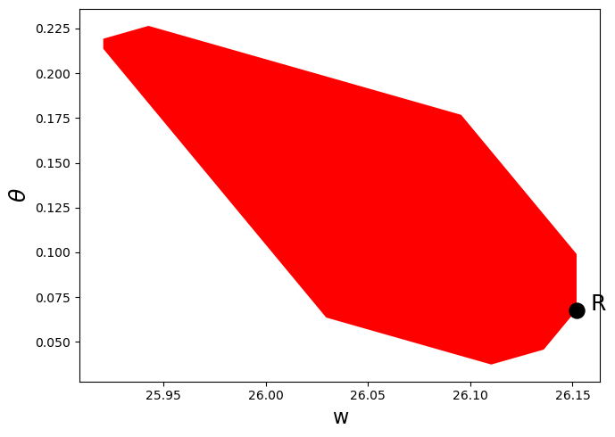
The remaining parameters ${β, \bar{m}, \underset{―}{h}, \bar{h}}$ are then variables to be specified for an instance of the Chang class.

Below we use the class to solve the model and plot the resulting equilibrium set, once with $β = 0.3$ and once with $β = 0.8$ .

(Here we have set the number of subgradients to 10 in order to speed up the code for now - we can increase accuracy by increasing the number of subgradients)

"""
Provides a class called ChangModel to solve different
parameterizations of the Chang (1998) model.
"""

import numpy as np
import time

from scipy.optimize import linprog, minimize
import numpy.polynomial.chebyshev as cheb


class ChangModel:
    """
    Class to solve for the competitive and sustainable sets in the Chang (1998)
    model, for different parameterizations.
    """

    def __init__(self, β, mbar, h_min, h_max, n_h, n_m, N_g):
        # Record parameters
        self.β, self.mbar, self.h_min, self.h_max = β, mbar, h_min, h_max
        self.n_h, self.n_m, self.N_g = n_h, n_m, N_g

        # Create other parameters
        self.m_min = 1e-9
        self.m_max = self.mbar
        self.N_a = self.n_h*self.n_m

        # Utility and production functions
        uc = lambda c: np.log(np.maximum(c, 1e-10))  # Clip to 1e-10 to avoid log(0) or log(-ve)
        uc_p = lambda c: 1/c
        v = lambda m: 1/500 * (mbar * m - 0.5 * m**2)**0.5
        v_p = lambda m: 0.5/500 * (mbar * m - 0.5 * m**2)**(-0.5) * (mbar - m)
        u = lambda h, m: uc(f(h, m)) + v(m)

        def f(h, m):
            x = m * (h - 1)
            f = 180 - (0.4 * x)**2
            return f

        def θ(h, m):
            x = m * (h - 1)
            θ = uc_p(f(h, m)) * (m + x)
            return θ

        # Create set of possible action combinations, A
        A1 = np.linspace(h_min, h_max, n_h).reshape(n_h, 1)
        A2 = np.linspace(self.m_min, self.m_max, n_m).reshape(n_m, 1)
        self.A = np.concatenate((np.kron(np.ones((n_m, 1)), A1),
                                 np.kron(A2, np.ones((n_h, 1)))), axis=1)

        # Pre-compute utility and output vectors
        self.euler_vec = -np.multiply(self.A[:, 1], \
            uc_p(f(self.A[:, 0], self.A[:, 1])) - v_p(self.A[:, 1]))
        self.u_vec = u(self.A[:, 0], self.A[:, 1])
        self.Θ_vec = θ(self.A[:, 0], self.A[:, 1])
        self.f_vec = f(self.A[:, 0], self.A[:, 1])
        self.bell_vec = np.multiply(uc_p(f(self.A[:, 0],
                                   self.A[:, 1])),
                                   np.multiply(self.A[:, 1],
                                   (self.A[:, 0] - 1))) \
                        + np.multiply(self.A[:, 1],
                                      v_p(self.A[:, 1]))

        # Find extrema of (w, θ) space for initial guess of equilibrium sets
        p_vec = np.zeros(self.N_a)
        w_vec = np.zeros(self.N_a)
        for i in range(self.N_a):
            p_vec[i] = self.Θ_vec[i]
            w_vec[i] = self.u_vec[i]/(1 - β)

        w_space = np.array([min(w_vec[~np.isinf(w_vec)]),
                            max(w_vec[~np.isinf(w_vec)])])
        p_space = np.array([0, max(p_vec[~np.isinf(w_vec)])])
        self.p_space = p_space

        # Set up hyperplane levels and gradients for iterations
        def SG_H_V(N, w_space, p_space):
            """
            This function  initializes the subgradients, hyperplane levels,
            and extreme points of the value set by choosing an appropriate
            origin and radius. It is based on a similar function in QuantEcon's
            Games.jl
            """

            # First, create a unit circle. Want points placed on [0, 2π]
            inc = 2 * np.pi / N
            degrees = np.arange(0, 2 * np.pi, inc)

            # Points on circle
            H = np.zeros((N, 2))
            for i in range(N):
                x = degrees[i]
                H[i, 0] = np.cos(x)
                H[i, 1] = np.sin(x)

            # Then calculate origin and radius
            o = np.array([np.mean(w_space), np.mean(p_space)])
            r1 = max((max(w_space) - o[0])**2, (o[0] - min(w_space))**2)
            r2 = max((max(p_space) - o[1])**2, (o[1] - min(p_space))**2)
            r = np.sqrt(r1 + r2)

            # Now calculate vertices
            Z = np.zeros((2, N))
            for i in range(N):
                Z[0, i] = o[0] + r*H.T[0, i]
                Z[1, i] = o[1] + r*H.T[1, i]

            # Corresponding hyperplane levels
            C = np.zeros(N)
            for i in range(N):
                C[i] = np.dot(Z[:, i], H[i, :])

            return C, H, Z

        C, self.H, Z = SG_H_V(N_g, w_space, p_space)
        C = C.reshape(N_g, 1)
        self.c0_c, self.c0_s, self.c1_c, self.c1_s = np.copy(C), np.copy(C), \
            np.copy(C), np.copy(C)
        self.z0_s, self.z0_c, self.z1_s, self.z1_c = np.copy(Z), np.copy(Z), \
            np.copy(Z), np.copy(Z)

        self.w_bnds_s, self.w_bnds_c = (w_space[0], w_space[1]), \
            (w_space[0], w_space[1])
        self.p_bnds_s, self.p_bnds_c = (p_space[0], p_space[1]), \
            (p_space[0], p_space[1])

        # Create dictionaries to save equilibrium set for each iteration
        self.c_dic_s, self.c_dic_c = {}, {}
        self.c_dic_s[0], self.c_dic_c[0] = self.c0_s, self.c0_c

    def solve_worst_spe(self):
        """
        Method to solve for BR(Z). See p.449 of Chang (1998)
        """

        p_vec = np.full(self.N_a, np.nan)
        c = [1, 0]

        # Pre-compute constraints
        aineq_mbar = np.vstack((self.H, np.array([0, -self.β])))
        bineq_mbar = np.vstack((self.c0_s, 0))

        aineq = self.H
        bineq = self.c0_s
        aeq = [[0, -self.β]]

        for j in range(self.N_a):
            # Only try if consumption is possible
            if self.f_vec[j] > 0:
                # If m = mbar, use inequality constraint
                if self.A[j, 1] == self.mbar:
                    bineq_mbar[-1] = self.euler_vec[j]
                    res = linprog(c, A_ub=aineq_mbar, b_ub=bineq_mbar,
                                  bounds=(self.w_bnds_s, self.p_bnds_s))
                else:
                    beq = self.euler_vec[j]
                    res = linprog(c, A_ub=aineq, b_ub=bineq, A_eq=aeq, b_eq=beq,
                                  bounds=(self.w_bnds_s, self.p_bnds_s))
                if res.status == 0:
                    p_vec[j] = self.u_vec[j] + self.β * res.x[0]

        # Max over h and min over other variables (see Chang (1998) p.449)
        self.br_z = np.nanmax(np.nanmin(p_vec.reshape(self.n_m, self.n_h), 0))

    def solve_subgradient(self):
        """
        Method to solve for E(Z). See p.449 of Chang (1998)
        """

        # Pre-compute constraints
        aineq_C_mbar = np.vstack((self.H, np.array([0, -self.β])))
        bineq_C_mbar = np.vstack((self.c0_c, 0))

        aineq_C = self.H
        bineq_C = self.c0_c
        aeq_C = [[0, -self.β]]

        aineq_S_mbar = np.vstack((np.vstack((self.H, np.array([0, -self.β]))),
                                  np.array([-self.β, 0])))
        bineq_S_mbar = np.vstack((self.c0_s, np.zeros((2, 1))))

        aineq_S = np.vstack((self.H, np.array([-self.β, 0])))
        bineq_S = np.vstack((self.c0_s, 0))
        aeq_S = [[0, -self.β]]

        # Update maximal hyperplane level
        for i in range(self.N_g):
            c_a1a2_c, t_a1a2_c = np.full(self.N_a, -np.inf), \
                np.zeros((self.N_a, 2))
            c_a1a2_s, t_a1a2_s = np.full(self.N_a, -np.inf), \
                np.zeros((self.N_a, 2))

            c = [-self.H[i, 0], -self.H[i, 1]]

            for j in range(self.N_a):
                # Only try if consumption is possible
                if self.f_vec[j] > 0:

                    # COMPETITIVE EQUILIBRIA
                    # If m = mbar, use inequality constraint
                    if self.A[j, 1] == self.mbar:
                        bineq_C_mbar[-1] = self.euler_vec[j]
                        res = linprog(c, A_ub=aineq_C_mbar, b_ub=bineq_C_mbar,
                                      bounds=(self.w_bnds_c, self.p_bnds_c))
                    # If m < mbar, use equality constraint
                    else:
                        beq_C = self.euler_vec[j]
                        res = linprog(c, A_ub=aineq_C, b_ub=bineq_C, A_eq = aeq_C,
                                      b_eq = beq_C, bounds=(self.w_bnds_c, \
                                          self.p_bnds_c))
                    if res.status == 0:
                        c_a1a2_c[j] = self.H[i, 0] * (self.u_vec[j] \
                            + self.β * res.x[0]) + self.H[i, 1] * self.Θ_vec[j]
                        t_a1a2_c[j] = res.x

                    # SUSTAINABLE EQUILIBRIA
                    # If m = mbar, use inequality constraint
                    if self.A[j, 1] == self.mbar:
                        bineq_S_mbar[-2] = self.euler_vec[j]
                        bineq_S_mbar[-1] = self.u_vec[j] - self.br_z
                        res = linprog(c, A_ub=aineq_S_mbar, b_ub=bineq_S_mbar,
                                      bounds=(self.w_bnds_s, self.p_bnds_s))
                    # If m < mbar, use equality constraint
                    else:
                        bineq_S[-1] = self.u_vec[j] - self.br_z
                        beq_S = self.euler_vec[j]
                        res = linprog(c, A_ub=aineq_S, b_ub=bineq_S, A_eq = aeq_S,
                                      b_eq = beq_S, bounds=(self.w_bnds_s, \
                                          self.p_bnds_s))
                    if res.status == 0:
                        c_a1a2_s[j] = self.H[i, 0] * (self.u_vec[j] \
                            + self.β*res.x[0]) + self.H[i, 1] * self.Θ_vec[j]
                        t_a1a2_s[j] = res.x

            idx_c = np.where(c_a1a2_c == max(c_a1a2_c))[0][0]
            self.z1_c[:, i] = np.array([self.u_vec[idx_c]
                                        + self.β * t_a1a2_c[idx_c, 0],
                                        self.Θ_vec[idx_c]])

            idx_s = np.where(c_a1a2_s == max(c_a1a2_s))[0][0]
            self.z1_s[:, i] = np.array([self.u_vec[idx_s]
                                        + self.β * t_a1a2_s[idx_s, 0],
                                        self.Θ_vec[idx_s]])

        for i in range(self.N_g):
            self.c1_c[i] = np.dot(self.z1_c[:, i], self.H[i, :])
            self.c1_s[i] = np.dot(self.z1_s[:, i], self.H[i, :])

    def solve_sustainable(self, tol=1e-5, max_iter=250):
        """
        Method to solve for the competitive and sustainable equilibrium sets.
        """

        t = time.time()
        diff = tol + 1
        iters = 0

        print('### --------------- ###')
        print('Solving Chang Model Using Outer Hyperplane Approximation')
        print('### --------------- ### \n')

        print('Maximum difference when updating hyperplane levels:')

        while diff > tol and iters < max_iter:
            iters = iters + 1
            self.solve_worst_spe()
            self.solve_subgradient()
            diff = max(np.maximum(abs(self.c0_c - self.c1_c),
                       abs(self.c0_s - self.c1_s)))
            print(diff)

            # Update hyperplane levels
            self.c0_c, self.c0_s = np.copy(self.c1_c), np.copy(self.c1_s)

            # Update bounds for w and θ
            wmin_c, wmax_c = np.min(self.z1_c, axis=1)[0], \
                np.max(self.z1_c, axis=1)[0]
            pmin_c, pmax_c = np.min(self.z1_c, axis=1)[1], \
                np.max(self.z1_c, axis=1)[1]

            wmin_s, wmax_s = np.min(self.z1_s, axis=1)[0], \
                np.max(self.z1_s, axis=1)[0]
            pmin_S, pmax_S = np.min(self.z1_s, axis=1)[1], \
                np.max(self.z1_s, axis=1)[1]

            self.w_bnds_s, self.w_bnds_c = (wmin_s, wmax_s), (wmin_c, wmax_c)
            self.p_bnds_s, self.p_bnds_c = (pmin_S, pmax_S), (pmin_c, pmax_c)

            # Save iteration
            self.c_dic_c[iters], self.c_dic_s[iters] = np.copy(self.c1_c), \
                np.copy(self.c1_s)
            self.iters = iters

        elapsed = time.time() - t
        print('Convergence achieved after {} iterations and {} \
            seconds'.format(iters, round(elapsed, 2)))

    def solve_bellman(self, θ_min, θ_max, order, disp=False, tol=1e-7, maxiters=100):
        """
        Continuous Method to solve the Bellman equation in section 25.3
        """
        mbar = self.mbar

        # Utility and production functions
        uc = lambda c: np.log(np.maximum(c, 1e-10))  # Clip to 1e-10 to avoid log(0) or log(-ve)
        uc_p = lambda c: 1 / c
        v = lambda m: 1 / 500 * (mbar * m - 0.5 * m**2)**0.5
        v_p = lambda m: 0.5/500 * (mbar*m - 0.5 * m**2)**(-0.5) * (mbar - m)
        u = lambda h, m: uc(f(h, m)) + v(m)

        def f(h, m):
            x = m * (h - 1)
            f = 180 - (0.4 * x)**2
            return f

        def θ(h, m):
            x = m * (h - 1)
            θ = uc_p(f(h, m)) * (m + x)
            return θ

        # Bounds for Maximization
        lb1 = np.array([self.h_min, 0, θ_min])
        ub1 = np.array([self.h_max, self.mbar - 1e-5, θ_max])
        lb2 = np.array([self.h_min, θ_min])
        ub2 = np.array([self.h_max, θ_max])

        # Initialize Value Function coefficients
        # Calculate roots of Chebyshev polynomial
        k = np.linspace(order, 1, order)
        roots = np.cos((2 * k - 1) * np.pi / (2 * order))
        # Scale to approximation space
        s = θ_min + (roots - -1) / 2 * (θ_max - θ_min)
        # Create a basis matrix
        Φ = cheb.chebvander(roots, order - 1)
        c = np.zeros(Φ.shape[0])

        # Function to minimize and constraints
        def p_fun(x):
            scale = -1 + 2 * (x[2] - θ_min)/(θ_max - θ_min)
            p_fun = - (u(x[0], x[1]) \
                + self.β * np.dot(cheb.chebvander(scale, order - 1), c))
            return p_fun.item()

        def p_fun2(x):
            scale = -1 + 2*(x[1] - θ_min)/(θ_max - θ_min)
            p_fun = - (u(x[0],mbar) \
                + self.β * np.dot(cheb.chebvander(scale, order - 1), c))
            return p_fun.item()

        cons1 = ({'type': 'eq',   'fun': lambda x: uc_p(f(x[0], x[1])) * x[1]
                    * (x[0] - 1) + v_p(x[1]) * x[1] + self.β * x[2] - θ},
                 {'type': 'eq',   'fun': lambda x: uc_p(f(x[0], x[1]))
                    * x[0] * x[1] - θ})
        cons2 = ({'type': 'ineq', 'fun': lambda x: uc_p(f(x[0], mbar)) * mbar
                    * (x[0] - 1) + v_p(mbar) * mbar + self.β * x[1] - θ},
                 {'type': 'eq',   'fun': lambda x: uc_p(f(x[0], mbar))
                    * x[0] * mbar - θ})

        bnds1 = np.concatenate([lb1.reshape(3, 1), ub1.reshape(3, 1)], axis=1)
        bnds2 = np.concatenate([lb2.reshape(2, 1), ub2.reshape(2, 1)], axis=1)

        # Bellman Iterations
        diff = 1
        iters = 1

        while diff > tol:
        # 1. Maximization, given value function guess
            p_iter1 = np.zeros(order)
            for i in range(order):
                θ = s[i]
                x0 = np.clip(lb1 + (ub1-lb1)/2, lb1, ub1)
                res = minimize(p_fun,
                               x0,
                               method='SLSQP',
                               bounds=bnds1,
                               constraints=cons1,
                               tol=1e-10)
                if res.success == True:
                    p_iter1[i] = -p_fun(res.x)
                x0 = np.clip(lb2 + (ub2-lb2)/2, lb2, ub2)
                res = minimize(p_fun2,
                               x0,
                               method='SLSQP',
                               bounds=bnds2,
                               constraints=cons2,
                               tol=1e-10)
                if -p_fun2(res.x) > p_iter1[i] and res.success == True:
                    p_iter1[i] = -p_fun2(res.x)

            # 2. Bellman updating of Value Function coefficients
            c1 = np.linalg.solve(Φ, p_iter1)
            # 3. Compute distance and update
            diff = np.linalg.norm(c - c1)
            if bool(disp == True):
                print(diff)
            c = np.copy(c1)
            iters = iters + 1
            if iters > maxiters:
                print('Convergence failed after {} iterations'.format(maxiters))
                break

        self.θ_grid = s
        self.p_iter = p_iter1
        self.Φ = Φ
        self.c = c
        print('Convergence achieved after {} iterations'.format(iters))

        # Check residuals
        θ_grid_fine = np.linspace(θ_min, θ_max, 100)
        resid_grid = np.zeros(100)
        p_grid = np.zeros(100)
        θ_prime_grid = np.zeros(100)
        m_grid = np.zeros(100)
        h_grid = np.zeros(100)
        for i in range(100):
            θ = θ_grid_fine[i]
            x0 = np.clip(lb1 + (ub1-lb1)/2, lb1, ub1)
            res = minimize(p_fun,
                           x0,
                           method='SLSQP',
                           bounds=bnds1,
                           constraints=cons1,
                           tol=1e-10)
            if res.success == True:
                p = -p_fun(res.x)
                p_grid[i] = p
                θ_prime_grid[i] = res.x[2]
                h_grid[i] = res.x[0]
                m_grid[i] = res.x[1]
            x0 = np.clip(lb2 + (ub2-lb2)/2, lb2, ub2)
            res = minimize(p_fun2,
                           x0,
                           method='SLSQP',
                           bounds=bnds2,
                           constraints=cons2,
                           tol=1e-10)
            if -p_fun2(res.x) > p and res.success == True:
                p = -p_fun2(res.x)
                p_grid[i] = p
                θ_prime_grid[i] = res.x[1]
                h_grid[i] = res.x[0]
                m_grid[i] = self.mbar
            scale = -1 + 2 * (θ - θ_min)/(θ_max - θ_min)
            resid_grid_val = np.dot(cheb.chebvander(scale, order-1), c) - p
            resid_grid[i] = resid_grid_val.item()

        self.resid_grid = resid_grid
        self.θ_grid_fine = θ_grid_fine
        self.θ_prime_grid = θ_prime_grid
        self.m_grid = m_grid
        self.h_grid = h_grid
        self.p_grid = p_grid
        self.x_grid = m_grid * (h_grid - 1)

        # Simulate
        θ_series = np.zeros(31)
        m_series = np.zeros(30)
        h_series = np.zeros(30)

        # Find initial θ
        def ValFun(x):
            scale = -1 + 2*(x - θ_min)/(θ_max - θ_min)
            p_fun = np.dot(cheb.chebvander(scale, order - 1), c)
            return -p_fun

        res = minimize(ValFun,
                      (θ_min + θ_max)/2,
                      bounds=[(θ_min, θ_max)])
        θ_series[0] = res.x.item()

        # Simulate
        for i in range(30):
            θ = θ_series[i]
            x0 = np.clip(lb1 + (ub1-lb1)/2, lb1, ub1)
            res = minimize(p_fun,
                           x0,
                           method='SLSQP',
                           bounds=bnds1,
                           constraints=cons1,
                           tol=1e-10)
            if res.success == True:
                p = -p_fun(res.x)
                h_series[i] = res.x[0]
                m_series[i] = res.x[1]
                θ_series[i+1] = res.x[2]
            x0 = np.clip(lb2 + (ub2-lb2)/2, lb2, ub2)
            res2 = minimize(p_fun2,
                            x0,
                            method='SLSQP',
                            bounds=bnds2,
                            constraints=cons2,
                            tol=1e-10)
            if -p_fun2(res2.x) > p and res2.success == True:
                h_series[i] = res2.x[0]
                m_series[i] = self.mbar
                θ_series[i+1] = res2.x[1]

        self.θ_series = θ_series
        self.m_series = m_series
        self.h_series = h_series
        self.x_series = m_series * (h_series - 1)

ch1 = ChangModel(β=0.3, mbar=30, h_min=0.9, h_max=2, n_h=8, n_m=35, N_g=10)
ch1.solve_sustainable()

### --------------- ###
Solving Chang Model Using Outer Hyperplane Approximation
### --------------- ### 

Maximum difference when updating hyperplane levels:

[1.9168]

[0.66782]

[0.49235]

[0.32412]

[0.19022]

[0.10863]

[0.05817]

[0.0262]

[0.01836]

[0.01415]

[0.00297]

[0.00089]

[0.00027]

[0.00008]

[0.00002]

[0.00001]
Convergence achieved after 16 iterations and 39.06             seconds

def plot_competitive(ChangModel):
    """
    Method that only plots competitive equilibrium set
    """
    poly_C = polytope.Polytope(ChangModel.H, ChangModel.c1_c)
    ext_C = polytope.extreme(poly_C)

    fig, ax = plt.subplots(figsize=(7, 5))

    ax.set_xlabel('w', fontsize=16)
    ax.set_ylabel(r"$\theta$", fontsize=18)

    ax.fill(ext_C[:,0], ext_C[:,1], 'r', zorder=0)
    ChangModel.min_theta = min(ext_C[:, 1])
    ChangModel.max_theta = max(ext_C[:, 1])

    # Add point showing Ramsey Plan
    idx_Ramsey = np.where(ext_C[:, 0] == max(ext_C[:, 0]))[0][0]
    R = ext_C[idx_Ramsey, :]
    ax.scatter(R[0], R[1], 150, 'black', marker='o', zorder=1)
    w_min = min(ext_C[:, 0])

    # Label Ramsey Plan slightly to the right of the point
    ax.annotate("R", xy=(R[0], R[1]), xytext=(R[0] + 0.03 * (R[0] - w_min),
                R[1]), fontsize=18)

    plt.tight_layout()
    plt.show()

plot_competitive(ch1)

_images/6ba3a5787f817641146360fa81e154677251a9786972d9f0eef1a42e5b02da40.png

ch2 = ChangModel(β=0.8, mbar=30, h_min=0.9, h_max=1/0.8,
                 n_h=8, n_m=35, N_g=10)
ch2.solve_sustainable()

### --------------- ###
Solving Chang Model Using Outer Hyperplane Approximation
### --------------- ### 

Maximum difference when updating hyperplane levels:

[0.06369]

[0.02476]

[0.02153]

[0.01915]

[0.01795]

[0.01642]

[0.01507]

[0.01284]

[0.01106]

[0.00694]

[0.0085]

[0.00781]

[0.00433]

[0.00492]

[0.00303]

[0.00182]

[0.00638]

[0.00116]

[0.00093]

[0.00075]

[0.0006]

[0.00494]

[0.00038]

[0.00121]

[0.00024]

[0.0002]

[0.00016]

[0.00013]

[0.0001]

[0.00008]

[0.00006]

[0.00005]

[0.00004]

[0.00003]

[0.00003]

[0.00002]

[0.00002]

[0.00001]

[0.00001]

[0.00001]
Convergence achieved after 40 iterations and 113.42             seconds

plot_competitive(ch2)

_images/74c5979c9b0d0383a126b0c00a4a8d2133326b96430b980e3c32d2aa8b40ebd2.png

49.7. Solving a Continuation Ramsey Planner’s Bellman Equation#

In this section we solve the Bellman equation confronting a continuation Ramsey planner.

The construction of a Ramsey plan is decomposed into a two subproblems in Ramsey plans, time inconsistency, sustainable plans and dynamic Stackelberg problems.

Subproblem 1 is faced by a sequence of continuation Ramsey planners at $t \geq 1$ .
Subproblem 2 is faced by a Ramsey planner at $t = 0$ .

The problem is:

J (θ) = max_{m, x, h, θ^{'}} u (f (x)) + v (m) + β J (θ^{'})

subject to:

θ \leq u^{'} (f (x)) x + v^{'} (m) m + β θ^{'}

θ = u^{'} (f (x)) (m + x)

x = m (h - 1)

(m, x, h) \in E

θ^{'} \in Ω

To solve this Bellman equation, we must know the set $Ω$ .

We have solved the Bellman equation for the two sets of parameter values for which we computed the equilibrium value sets above.

Hence for these parameter configurations, we know the bounds of $Ω$ .

The two sets of parameters differ only in the level of $β$ .

From the figures earlier in this lecture, we know that when $β = 0.3$ , $Ω = [0.0088, 0.0499]$ , and when $β = 0.8$ , $Ω = [0.0395, 0.2193]$

ch1 = ChangModel(β=0.3, mbar=30, h_min=0.99, h_max=1/0.3,
                 n_h=8, n_m=35, N_g=50)
ch2 = ChangModel(β=0.8, mbar=30, h_min=0.1, h_max=1/0.8,
                 n_h=20, n_m=50, N_g=50)

ch1.solve_bellman(θ_min=0.01, θ_max=0.0499, order=30, tol=1e-6)
ch2.solve_bellman(θ_min=0.045, θ_max=0.15, order=30, tol=1e-6)

Convergence achieved after 15 iterations

/home/runner/miniconda3/envs/quantecon/lib/python3.12/site-packages/scipy/optimize/_slsqp_py.py:437: RuntimeWarning: Values in x were outside bounds during a minimize step, clipping to bounds
  fx = wrapped_fun(x)

/home/runner/miniconda3/envs/quantecon/lib/python3.12/site-packages/scipy/optimize/_slsqp_py.py:441: RuntimeWarning: Values in x were outside bounds during a minimize step, clipping to bounds
  g = append(wrapped_grad(x), 0.0)
/home/runner/miniconda3/envs/quantecon/lib/python3.12/site-packages/scipy/optimize/_slsqp_py.py:495: RuntimeWarning: Values in x were outside bounds during a minimize step, clipping to bounds
  a_eq = vstack([con['jac'](x, *con['args'])
/home/runner/miniconda3/envs/quantecon/lib/python3.12/site-packages/scipy/optimize/_slsqp_py.py:501: RuntimeWarning: Values in x were outside bounds during a minimize step, clipping to bounds
  a_ieq = vstack([con['jac'](x, *con['args'])

Convergence achieved after 72 iterations

First, a quick check that our approximations of the value functions are good.

We do this by calculating the residuals between iterates on the value function on a fine grid:

max(abs(ch1.resid_grid)), max(abs(ch2.resid_grid))

(6.46313155971967e-06, 6.875358415925348e-07)

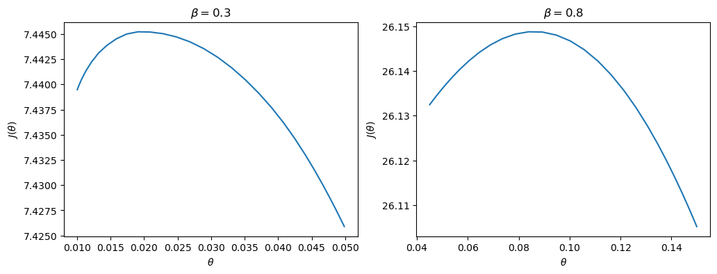
The value functions plotted below trace out the right edges of the sets of equilibrium values plotted above

fig, axes = plt.subplots(1, 2, figsize=(12, 4))

for ax, model in zip(axes, (ch1, ch2)):
    ax.plot(model.θ_grid, model.p_iter)
    ax.set(xlabel=r"$\theta$",
           ylabel=r"$J(\theta)$",
           title=rf"$\beta = {model.β}$")

plt.show()

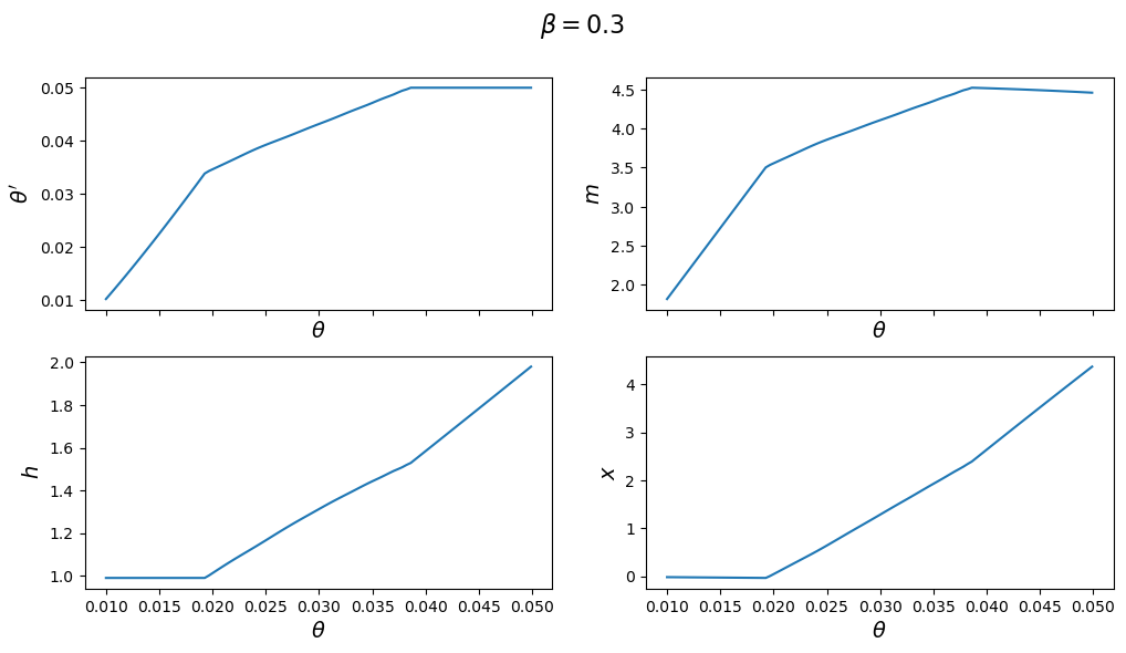
_images/60559012f92be5ff3858421e749bb4d76d38854ba8eb7dd9e22281e967ca126b.png

The next figure plots the optimal policy functions; values of $θ^{'}, m, x, h$ for each value of the state $θ$ :

for model in (ch1, ch2):

    fig, axes = plt.subplots(2, 2, figsize=(12, 6), sharex=True)
    fig.suptitle(rf"$\beta = {model.β}$", fontsize=16)

    plots = [model.θ_prime_grid, model.m_grid,
             model.h_grid, model.x_grid]
    labels = [r"$\theta'$", "$m$", "$h$", "$x$"]

    for ax, plot, label in zip(axes.flatten(), plots, labels):
        ax.plot(model.θ_grid_fine, plot)
        ax.set_xlabel(r"$\theta$", fontsize=14)
        ax.set_ylabel(label, fontsize=14)

    plt.show()

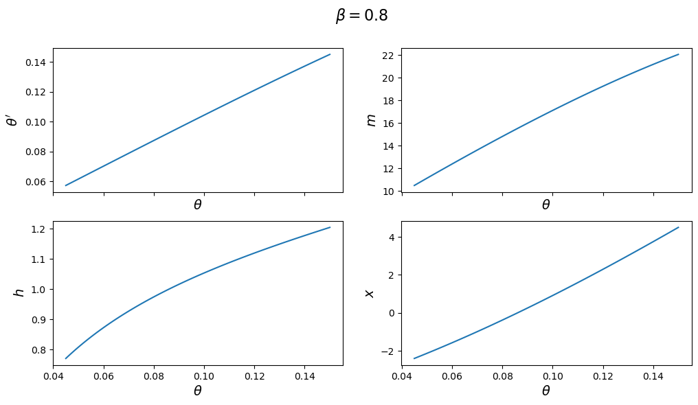
_images/d30f42d22d85febd08d709b86a4a78cf0002072ac924a915175b8d5c95eff3c9.png

_images/14f53e80a45262a21d12bcb7498696a59f498ca21f4ff7742ff91e9295f7e410.png

With the first set of parameter values, the value of $θ^{'}$ chosen by the Ramsey planner quickly hits the upper limit of $Ω$ .

But with the second set of parameters it converges to a value in the interior of the set.

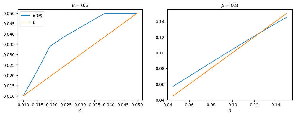
Consequently, the choice of $\bar{θ}$ is clearly important with the first set of parameter values.

One way of seeing this is plotting $θ^{'} (θ)$ for each set of parameters.

With the first set of parameter values, this function does not intersect the 45-degree line until $\bar{θ}$ , whereas in the second set of parameter values, it intersects in the interior.

fig, axes = plt.subplots(1, 2, figsize=(12, 4))

for ax, model in zip(axes, (ch1, ch2)):
    ax.plot(model.θ_grid_fine, model.θ_prime_grid, label=r"$\theta'(\theta)$")
    ax.plot(model.θ_grid_fine, model.θ_grid_fine, label=r"$\theta$")
    ax.set(xlabel=r"$\theta$", title=rf"$\beta = {model.β}$")

axes[0].legend()
plt.show()

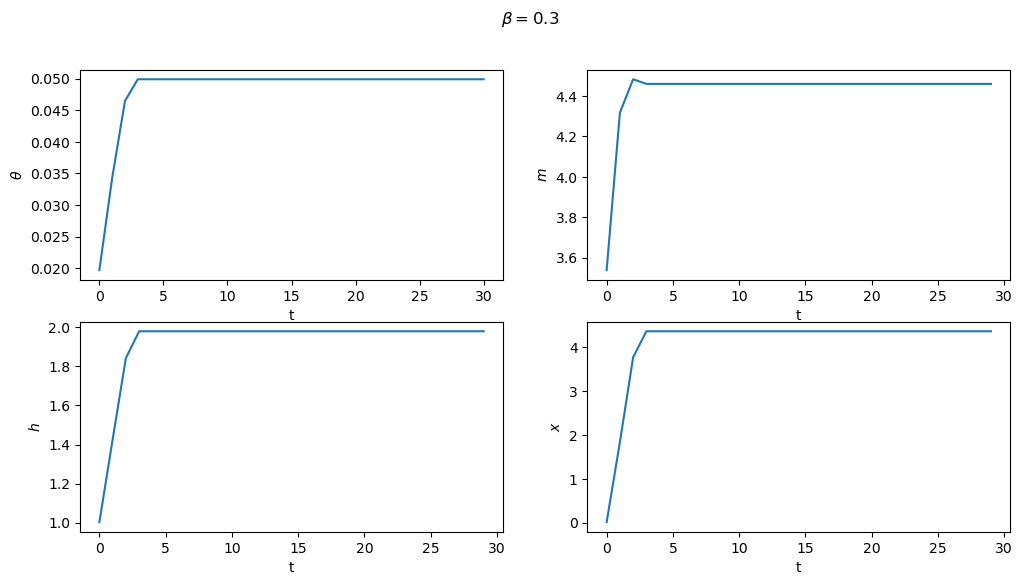
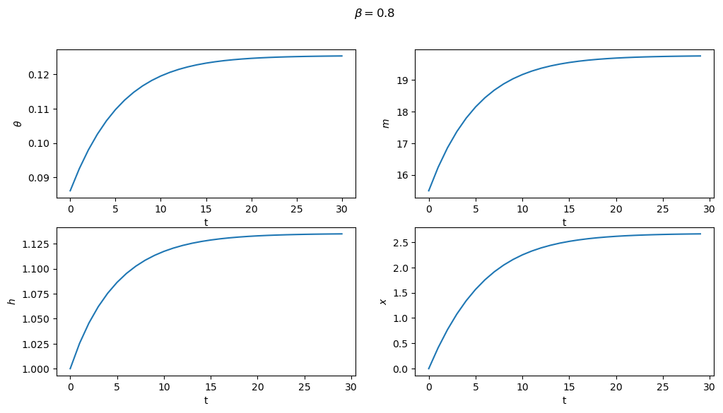
_images/e6dcd0496b629ac06adaa3d2306418af04fe4ffaf653af5143df070452c51da8.png

Subproblem 2 is equivalent to the planner choosing the initial value of $θ$ (i.e. the value which maximizes the value function).

From this starting point, we can then trace out the paths for ${θ_{t}, m_{t}, h_{t}, x_{t}}_{t = 0}^{\infty}$ that support this equilibrium.

These are shown below for both sets of parameters

for model in (ch1, ch2):

    fig, axes = plt.subplots(2, 2, figsize=(12, 6))
    fig.suptitle(rf"$\beta = {model.β}$")

    plots = [model.θ_series, model.m_series, model.h_series, model.x_series]
    labels = [r"$\theta$", "$m$", "$h$", "$x$"]

    for ax, plot, label in zip(axes.flatten(), plots, labels):
        ax.plot(plot)
        ax.set(xlabel='t', ylabel=label)

    plt.show()

_images/07bb5aeabba2af31d2df99e36231fffa21479de067134415f9970debd1c9fdc3.png

_images/7acc0e96ba788b1b90b808fb7cfab099e53678d24c76ab819fab690ee61f050e.png

49.7.1. Next Steps#

In Credible Government Policies in Chang Model we shall find a subset of competitive equilibria that are sustainable in the sense that a sequence of government administrations that chooses sequentially, rather than once and for all at time $0$ will choose to implement them.

In the process of constructing them, we shall construct another, smaller set of competitive equilibria.