5. Information and Consumption Smoothing#

In addition to what’s in Anaconda, this lecture employs the following libraries:

!pip install --upgrade quantecon

5.1. Overview#

In the linear-quadratic permanent income of consumption smoothing model described in this quantecon lecture, a scalar parameter $β \in (0, 1)$ plays two roles:

it is a discount factor that the consumer applies to future utilities from consumption
it is the reciprocal of the gross interest rate on risk-free one-period loans

That $β$ plays these two roles is essential in delivering the outcome that, regardless of the stochastic process that describes his non-financial income, the consumer chooses to make consumption follow a random walk (see [Hall, 1978]).

In this lecture, we assign a third role to $β$ :

it describes a first-order moving average process for the growth in non-financial income

5.1.1. Same non-financial incomes, different information#

We study two consumers who have exactly the same nonfinancial income process and who both conform to the linear-quadratic permanent income of consumption smoothing model described here.

The two consumers have different information about their future nonfinancial incomes.

A better informed consumer each period receives news in the form of a shock that simultaneously affects both today’s nonfinancial income and the present value of future nonfinancial incomes in a particular way.

A less informed consumer each period receives a shock that equals the part of today’s nonfinancial income that could not be forecast from past values of nonfinancial income.

Even though they receive exactly the same nonfinancial incomes each period, our two consumers behave differently because they have different information about their future nonfinancial incomes.

The second consumer receives less information about future nonfinancial incomes in a sense that we shall make precise.

This difference in their information sets manifests itself in their responding differently to what they regard as time $t$ information shocks.

Thus, although at each date they receive exactly the same histories of nonfinancial income, our two consumers receive different shocks or news about their future nonfinancial incomes.

We use the different behaviors of our consumers as a way to learn about

operating characteristics of a linear-quadratic permanent income model
how the Kalman filter introduced in this lecture and/or another representation of the theory of optimal forecasting introduced in this lecture embody lessons that can be applied to the news and noise literature
ways of representing and computing optimal decision rules in the linear-quadratic permanent income model
a Ricardian equivalence outcome that describes effects on optimal consumption of a tax cut at time $t$ accompanied by a foreseen permanent increases in taxes that is just sufficient to cover the interest payments used to service the risk-free government bonds that are issued to finance the tax cut
a simple application of alternative ways to factor a covariance generating function along lines described in this lecture

This lecture can be regarded as an introduction to invertibility issues that take center stage in the analysis of fiscal foresight by Eric Leeper, Todd Walker, and Susan Yang [Leeper et al., 2013], as well as in chapter 4 of [Sargent et al., 1991].

5.2. Two Representations of One Nonfinancial Income Process#

We study consequences of endowing a consumer with one of two alternative representations for the change in the consumer’s nonfinancial income $y_{t + 1} - y_{t}$ .

For both types of consumer, a parameter $β \in (0, 1)$ plays three roles.

It appears

as a discount factor applied to future expected one-period utilities,
as the reciprocal of a gross interest rate on one-period loans, and
as a parameter in a first-order moving average that equals the increment in a consumer’s non-financial income

The first representation, which we shall sometimes refer to as the more informative representation, is

(5.1)#

y_{t + 1} - y_{t} = ε_{t + 1} - β^{- 1} ε_{t}

where ${ε_{t}}$ is an i.i.d. normally distributed scalar process with means of zero and contemporaneous variances $σ_{ε}^{2}$ .

This representation of the process is used by a consumer who at time $t$ knows both $y_{t}$ and the shock $ε_{t}$ and can use both of them to forecast future $y_{t + j}$ ’s.

As we’ll see below, representation (5.1) has the peculiar property that a positive shock $ε_{t + 1}$ leaves the discounted present value of the consumer’s financial income at time $t + 1$ unaltered.

The second representation of the same ${y_{t}}$ process is

(5.2)#

y_{t + 1} - y_{t} = a_{t + 1} - β a_{t}

where ${a_{t}}$ is another i.i.d. normally distributed scalar process, with means of zero and now variances $σ_{a}^{2} > σ_{ε}^{2}$ .

The i.i.d. shock variances are related by

σ_{a}^{2} = β^{- 2} σ_{ε}^{2} > σ_{ε}^{2}

so that the variance of the innovation exceeds the variance of the original shock by a multiplicative factor $β^{- 2}$ .

Representation (5.2) is the innovations representation of equation (5.1) associated with Kalman filtering theory.

To see how this works, note that equating representations (5.1) and (5.2) for $y_{t + 1} - y_{t}$ implies $ε_{t + 1} - β^{- 1} ε_{t} = a_{t + 1} - β a_{t}$ , which in turn implies

a_{t + 1} = β a_{t} + ε_{t + 1} - β^{- 1} ε_{t} .

Solving this difference equation backwards for $a_{t + 1}$ gives, after a few lines of algebra,

(5.3)#

a_{t + 1} = ε_{t + 1} + (β - β^{- 1}) \sum_{j = 0}^{\infty} β^{j} ε_{t - j}

which we can also write as

a_{t + 1} = \sum_{j = 0}^{\infty} h_{j} ε_{t + 1 - j} \equiv h (L) ε_{t + 1}

where $L$ is the one-period lag operator, $h (L) = \sum_{j = 0}^{\infty} h_{j} L^{j}$ , $I$ is the identity operator, and

h (L) = \frac{I - β^{- 1} L}{I - β L}

Let $g_{j} \equiv E z_{t} z_{t - j}$ be the $j$ th autocovariance of the ${y_{t} - y_{t - 1}}$ process.

Using calculations in the quantecon lecture, where $z \in C$ is a complex variable, the covariance generating function $g (z) = \sum_{j = - \infty}^{\infty} g_{j} z^{j}$ of the ${y_{t} - y_{t - 1}}$ process equals

g (z) = σ_{ε}^{2} h (z) h (z^{- 1}) = β^{- 2} σ_{ε}^{2} > σ_{ε}^{2},

which confirms that ${a_{t}}$ is a serially uncorrelated process with variance

σ_{a}^{2} = β^{- 1} σ_{ε}^{2} .

To verify these claims, just notice that $g (z) = β^{- 2} σ_{ε}^{2}$ implies that

$g_{0} = β^{- 2} σ_{ε}^{2}$ , and
$g_{j} = 0$ for $j \neq 0$ .

Alternatively, if you are uncomfortable with covariance generating functions, note that we can directly calculate $σ_{a}^{2}$ from formula (5.3) according to

σ_{a}^{2} = σ_{ε}^{2} + [1 + (β - β^{- 1})^{2} \sum_{j = 0}^{\infty} β^{2 j}] = β^{- 1} σ_{ε}^{2} .

5.3. Application of Kalman filter#

We can also use the the Kalman filter to obtain representation (5.2) from representation (5.1).

Thus, from equations associated with the Kalman filter, it can be verified that the steady-state Kalman gain $K = β^{2}$ and the steady state conditional covariance

Σ = E [(ε_{t} - {\hat{ε}}_{t})^{2} | y_{t - 1}, y_{t - 2}, \dots] = (1 - β^{2}) σ_{ε}^{2}

In a little more detail, let $z_{t} = y_{t} - y_{t - 1}$ and form the state-space representation

\begin{aligned} ε_{t + 1} & = 0 ε_{t} + ε_{t + 1} \\ z_{t + 1} & = - β^{- 1} ε_{t} + ε_{t + 1} \end{aligned}

and assume that $σ_{ε} = 1$ for convenience

Let’s compute the steady-state Kalman filter for this system.

Let $K$ be the steady-state gain and $a_{t + 1}$ the one-step ahead innovation.

The steady-state innovations representation is

\begin{aligned} {\hat{ε}}_{t + 1} & = 0 {\hat{ε}}_{t} + K a_{t + 1} \\ z_{t + 1} & = - β a_{t} + a_{t + 1} \end{aligned}

By applying formulas for the steady-state Kalman filter, by hand it is possible to verify that $K = β^{2}, σ_{a}^{2} = β^{- 2} σ_{ε}^{2} = β^{- 2},$ and $Σ = (1 - β^{2}) σ_{ε}^{2}$ .

Alternatively, we can obtain these formulas via the classical filtering theory described in this lecture.

5.4. News Shocks and Less Informative Shocks#

Representation (5.1) is cast in terms of a news shock $ε_{t + 1}$ that represents a shock to nonfinancial income coming from taxes, transfers, and other random sources of income changes known to a well-informed person who perhaps has all sorts of information about the income process.

Representation (5.2) for the same income process is driven by shocks $a_{t}$ that contain less information than the news shock $ε_{t}$ .

Representation (5.2) is called the innovations representation for the ${y_{t} - y_{t - 1}}$ process.

It is cast in terms of what time series statisticians call the innovation or fundamental shock that emerges from applying the theory of optimally predicting nonfinancial income based solely on the information in past levels of growth in nonfinancial income.

Fundamental for the $y_{t}$ process means that the shock $a_{t}$ can be expressed as a square-summable linear combination of $y_{t}, y_{t - 1}, \dots$ .

The shock $ε_{t}$ is not fundamental because it has more information about the future of the ${y_{t} - y_{t - 1}}$ process than is contained in $a_{t}$ .

Representation (5.3) reveals the important fact that the original shock $ε_{t}$ contains more information about future $y$ ’s than is contained in the semi-infinite history $y^{t} = [y_{t}, y_{t - 1}, \dots]$ .

Staring at representation (5.3) for $a_{t + 1}$ shows that it consists both of new news $ε_{t + 1}$ as well as a long moving average $(β - β^{- 1}) \sum_{j = 0}^{\infty} β^{j} ε_{t - j}$ of old news.

The more information representation (5.1) asserts that a shock $ε_{t}$ results in an impulse response to nonfinancial income of $ε_{t}$ times the sequence

1, 1 - β^{- 1}, 1 - β^{- 1}, \dots

so that a shock that increases nonfinancial income $y_{t}$ by $ε_{t}$ at time $t$ is followed by a change in future $y$ of $ε_{t}$ times $1 - β^{- 1} < 0$ in all subsequent periods.

Because $1 - β^{- 1} < 0$ , this means that a positive shock of $ε_{t}$ today raises income at time $t$ by $ε_{t}$ and then permanently decreases all future incomes by $(β^{- 1} - 1) ε_{t}$ .

This pattern precisely describes the following mental experiment:

The consumer receives a government transfer of $ε_{t}$ at time $t$ .
The government finances the transfer by issuing a one-period bond on which it pays a gross one-period risk-free interest rate equal to $β^{- 1}$ .
In each future period, the government rolls over the one-period bond and so continues to borrow $ε_{t}$ forever.
The government imposes a lump-sum tax on the consumer in order to pay just the current interest on the original bond and its rolled over successors.
Thus, in periods $t + 1, t + 2, \dots$ , the government levies a lump-sum tax on the consumer of $β^{- 1} - 1$ that is just enough to pay the interest on the bond.

The present value of the impulse response or moving average coefficients equals $d_{ε} (L) = \frac{0}{1 - β} = 0$ , a fact that we’ll see again below.

Representation (5.2), i.e., the innovations representation, asserts that a shock $a_{t}$ results in an impulse response to nonfinancial income of $a_{t}$ times

1, 1 - β, 1 - β, \dots

so that a shock that increases income $y_{t}$ by $a_{t}$ at time $t$ can be expected to be followed by an increase in $y_{t + j}$ of $a_{t}$ times $1 - β > 0$ in all future periods $j = 1, 2, \dots$ .

The present value of the impulse response or moving average coefficients for representation (5.2) is $d_{a} (β) = \frac{1 - β^{2}}{1 - β} = (1 + β)$ , another fact that will be important below.

5.5. Representation of $ε_{t}$ Shock in Terms of Future $y_{t}$ #

Notice that reprentation (5.1), namely, $y_{t + 1} - y_{t} = - β^{- 1} ε_{t} + ε_{t + 1}$ implies the linear difference equation

ε_{t} = β ε_{t + 1} - β (y_{t + 1} - y_{t}) .

Solving forward we obtain

ε_{t} = β (y_{t} - (1 - β) \sum_{j = 0}^{\infty} β^{j} y_{t + j + 1})

This equation shows that $ε_{t}$ equals $β$ times the one-step-backwards error in optimally backcasting $y_{t}$ based on the semi-infinite future $y_{+}^{t} \equiv [y_{t + 1}, y_{t + 2}, \dots]$ via the optimal backcasting formula

E [y_{t} | y_{+}^{t}] = (1 - β) \sum_{j = 0}^{\infty} β^{j} y_{t + j + 1}

Thus, $ε_{t}$ exactly reveals the gap between $y_{t}$ and $E [y_{t} | y_{+}^{t}]$ .

5.6. Representation in Terms of $a_{t}$ Shocks#

Next notice that representation (5.2), namely, $y_{t + 1} - y_{t} = - β a_{t} + a_{t + 1}$ implies the linear difference equation

a_{t + 1} = β a_{t} + (y_{t + 1} - y_{t})

Solving this equation backward establishes that the one-step-prediction error $a_{t + 1}$ is

a_{t + 1} = y_{t + 1} - (1 - β) \sum_{j = 0}^{\infty} β^{j} y_{t - j} .

Here the information set is $y^{t} = [y_{t}, y_{t - 1}, \dots]$ and a one step-ahead optimal prediction is

E [y_{t + 1} | y^{t}] = (1 - β) \sum_{j = 0}^{\infty} β^{j} y_{t - j}

5.7. Permanent Income Consumption-Smoothing Model#

When we computed optimal consumption-saving policies for our two representations (5.1) and (5.2) by using formulas obtained with the difference equation approach described in quantecon lecture, we obtained:

for a consumer having the information assumed in the news representation (5.1):

\begin{aligned} c_{t + 1} - c_{t} & = 0 \\ b_{t + 1} - b_{t} & = - β^{- 1} ε_{t} \end{aligned}

for a consumer having the more limited information associated with the innovations representation (5.2):

\begin{aligned} c_{t + 1} - c_{t} & = (1 - β^{2}) a_{t + 1} \\ b_{t + 1} - b_{t} & = - β a_{t} \end{aligned}

These formulas agree with outcomes from Python programs below that deploy state-space representations and dynamic programming.

Evidently, although they receive exactly the same histories of nonfinancial incomethe two consumers behave differently.

The better informed consumer who has the information sets associated with representation (5.1) responds to each shock $ε_{t + 1}$ by leaving his consumption unaltered and saving all of $ε_{t + 1}$ in anticipation of the permanently increased taxes that he will bear in order to service the permanent interest payments on the risk-free bonds that the government has presumably issued to pay for the one-time addition $ε_{t + 1}$ to his time $t + 1$ nonfinancial income.

The less well informed consumer who has information sets associated with representation (5.2) responds to a shock $a_{t + 1}$ by increasing his consumption by what he perceives to be the permanent part of the increase in consumption and by increasing his saving by what he perceives to be the temporary part.

The behavior of the better informed consumer sharply illustrates the behavior predicted in a classic Ricardian equivalence experiment.

5.8. State Space Representations#

We now cast our representations (5.1) and (5.2), respectively, in terms of the following two state space systems:

(5.4)#

\begin{aligned} [\begin{array}{c} y_{t + 1} \\ ε_{t + 1} \end{array}] & = [\begin{array}{c} 1 & - β^{- 1} \\ 0 & 0 \end{array}] [\begin{array}{c} y_{t} \\ ε_{t} \end{array}] + [\begin{array}{c} σ_{ε} \\ σ_{ε} \end{array}] v_{t + 1} \\ y_{t} & = [\begin{array}{c} 1 & 0 \end{array}] [\begin{array}{c} y_{t} \\ ε_{t} \end{array}] \end{aligned}

and

(5.5)#

\begin{aligned} [\begin{array}{c} y_{t + 1} \\ a_{t + 1} \end{array}] & = [\begin{array}{c} 1 & - β \\ 0 & 0 \end{array}] [\begin{array}{c} y_{t} \\ a_{t} \end{array}] + [\begin{array}{c} σ_{a} \\ σ_{a} \end{array}] u_{t + 1} \\ y_{t} & = [\begin{array}{c} 1 & 0 \end{array}] [\begin{array}{c} y_{t} \\ a_{t} \end{array}] \end{aligned}

where ${v_{t}}$ and ${u_{t}}$ are both i.i.d. sequences of univariate standardized normal random variables.

These two alternative income processes are ready to be used in the framework presented in the section “Comparison with the Difference Equation Approach” in thid quantecon lecture.

All the code that we shall use below is presented in that lecture.

5.9. Computations#

We shall use Python to form two state-space representations (5.4) and (5.5).

We set the following parameter values $σ_{ε} = 1, σ_{a} = β^{- 1} σ_{ε} = β^{- 1}$ where $β$ is the same value as the discount factor in the household’s problem in the LQ savings problem in the lecture.

For these two representations, we use the code in this lecture to

compute optimal decision rules for $c_{t}, b_{t}$ for the two types of consumers associated with our two representations of nonfinancial income
use the value function objects $P, d$ returned by the code to compute optimal values for the two representations when evaluated at the initial condition

x_{0} = [\begin{matrix} 10 \\ 0 \end{matrix}]

for each representation.

create instances of the LinearStateSpace class for the two representations of the ${y_{t}}$ process and use them to obtain impulse response functions of $c_{t}$ and $b_{t}$ to the respective shocks $ε_{t}$ and $a_{t}$ for the two representations.
run simulations of ${y_{t}, c_{t}, b_{t}}$ of length $T$ under both of the representations

We formulae the problem:

min \sum_{t = 0}^{\infty} β^{t} {(c_{t} - γ)}^{2}

subject to a sequence of constraints

c_{t} + b_{t} = \frac{1}{1 + r} b_{t + 1} + y_{t}, t \geq 0

where $y_{t}$ follows one of the representations defined above.

Define the control as $u_{t} \equiv c_{t} - γ$ .

(For simplicity we can assume $γ = 0$ below because $γ$ has no effect on the impulse response functions that interest us.)

The state transition equations under our two representations for the nonfinancial income process ${y_{t}}$ can be written as

\begin{array}{r} [\begin{array}{c} y_{t + 1} \\ ε_{t + 1} \\ b_{t + 1} \end{array}] = \underset{\equiv A_{1}}{\underset{⏟}{[\begin{array}{ccc} 1 & - β^{- 1} & 0 \\ 0 & 0 & 0 \\ - (1 + r) & 0 & 1 + r \end{array}]}} [\begin{array}{c} y_{t} \\ ε_{t} \\ b_{t} \end{array}] + \underset{\equiv B_{1}}{\underset{⏟}{[\begin{array}{c} 0 \\ 0 \\ 1 + r \end{array}]}} [\begin{array}{c} c_{t} \end{array}] + \underset{\equiv C_{1}}{\underset{⏟}{[\begin{array}{c} σ_{ε} \\ σ_{ε} \\ 0 \end{array}]}} ν_{t + 1}, \end{array}

and

\begin{array}{r} [\begin{array}{c} y_{t + 1} \\ a_{t + 1} \\ b_{t + 1} \end{array}] = \underset{\equiv A_{2}}{\underset{⏟}{[\begin{array}{ccc} 1 & - β & 0 \\ 0 & 0 & 0 \\ - (1 + r) & 0 & 1 + r \end{array}]}} [\begin{array}{c} y_{t} \\ a_{t} \\ b_{t} \end{array}] + \underset{\equiv B_{2}}{\underset{⏟}{[\begin{array}{c} 0 \\ 0 \\ 1 + r \end{array}]}} [\begin{array}{c} c_{t} \end{array}] + \underset{\equiv C_{2}}{\underset{⏟}{[\begin{array}{c} σ_{a} \\ σ_{a} \\ 0 \end{array}]}} u_{t + 1} . \end{array}

As usual, we start by importing packages.

import numpy as np
import quantecon as qe
import matplotlib.pyplot as plt

# Set parameters
β, σϵ = 0.95, 1
σa = σϵ / β

R = 1 / β

# Payoff matrices are the same for two representations
RLQ = np.array([[0, 0, 0],
                [0, 0, 0],
                [0, 0, 1e-12]]) # put penalty on debt
QLQ = np.array([1.])

# More informative representation state transition matrices
ALQ1 = np.array([[1, -R, 0],
                 [0, 0, 0],
                 [-R, 0, R]])
BLQ1 = np.array([[0, 0, R]]).T
CLQ1 = np.array([[σϵ, σϵ, 0]]).T

# Construct and solve the LQ problem
LQ1 = qe.LQ(QLQ, RLQ, ALQ1, BLQ1, C=CLQ1, beta=β)
P1, F1, d1 = LQ1.stationary_values()

# The optimal decision rule for c
-F1

array([[ 1.  , -1.  , -0.05]])

Evidently, optimal consumption and debt decision rules for the consumer having news representation (5.1) are

\begin{array}{r} \begin{aligned} c_{t}^{*} & = y_{t} - ε_{t} - (1 - β) b_{t}, \\ b_{t + 1}^{*} & = β^{- 1} c_{t}^{*} + β^{- 1} b_{t} - β^{- 1} y_{t} \\ = β^{- 1} y_{t} - β^{- 1} ε_{t} - (β^{- 1} - 1) b_{t} + β^{- 1} b_{t} - β^{- 1} y_{t} \\ = b_{t} - β^{- 1} ε_{t} . \end{aligned} \end{array}

# Innovations representation
ALQ2 = np.array([[1, -β, 0],
                 [0,  0, 0],
                 [-R, 0, R]])
BLQ2 = np.array([[0, 0, R]]).T
CLQ2 = np.array([[σa, σa, 0]]).T

LQ2 = qe.LQ(QLQ, RLQ, ALQ2, BLQ2, C=CLQ2, beta=β)
P2, F2, d2 = LQ2.stationary_values()

-F2

array([[ 1.    , -0.9025, -0.05  ]])

For a consumer having access only to the information associated with the innovations representation (5.2), the optimal decision rules are

\begin{array}{r} \begin{aligned} c_{t}^{*} & = y_{t} - β^{2} a_{t} - (1 - β) b_{t}, \\ b_{t + 1}^{*} & = β^{- 1} c_{t}^{*} + β^{- 1} b_{t} - β^{- 1} y_{t} \\ = β^{- 1} y_{t} - β a_{t} - (β^{- 1} - 1) b_{t} + β^{- 1} b_{t} - β^{- 1} y_{t} \\ = b_{t} - β a_{t} . \end{aligned} \end{array}

Now we construct two Linear State Space models that emerge from using optimal policies of the form $u_{t} = - F x_{t}$ .

Take the more informative original representation (5.1) as an example:

\begin{array}{r} [\begin{array}{c} y_{t + 1} \\ ε_{t + 1} \\ b_{t + 1} \end{array}] = (A_{1} - B_{1} F_{1}) [\begin{array}{c} y_{t} \\ ε_{t} \\ b_{t} \end{array}] + C_{1} ν_{t + 1} \end{array}

\begin{array}{r} [\begin{array}{c} c_{t} \\ b_{t} \end{array}] = [\begin{array}{c} - F_{1} \\ S_{b} \end{array}] [\begin{array}{c} y_{t} \\ ε_{t} \\ b_{t} \end{array}] \end{array}

To have the Linear State Space model be of an innovations representation form (5.2), we can simply replace the corresponding matrices.

# Construct two Linear State Space models
Sb = np.array([0, 0, 1])

ABF1 = ALQ1 - BLQ1 @ F1
G1 = np.vstack([-F1, Sb])
LSS1 = qe.LinearStateSpace(ABF1, CLQ1, G1)

ABF2 = ALQ2 - BLQ2 @ F2
G2 = np.vstack([-F2, Sb])
LSS2 = qe.LinearStateSpace(ABF2, CLQ2, G2)

The following code computes impulse response functions of $c_{t}$ and $b_{t}$ .

J = 5 # Number of coefficients that we want

x_res1, y_res1 = LSS1.impulse_response(j=J)
b_res1 = np.array([x_res1[i][2, 0] for i in range(J)])
c_res1 = np.array([y_res1[i][0, 0] for i in range(J)])

x_res2, y_res2 = LSS2.impulse_response(j=J)
b_res2 = np.array([x_res2[i][2, 0] for i in range(J)])
c_res2 = np.array([y_res2[i][0, 0] for i in range(J)])

c_res1 / σϵ, b_res1 / σϵ

(array([1.99998906e-11, 1.89473923e-11, 1.78947621e-11, 1.68421319e-11,
        1.57895017e-11]),
 array([ 0.        , -1.05263158, -1.05263158, -1.05263158, -1.05263158]))

plt.title("more informative representation")
plt.plot(range(J), c_res1 / σϵ, label="c impulse response function")
plt.plot(range(J), b_res1 / σϵ, label="b impulse response function")
plt.legend()

<matplotlib.legend.Legend at 0x7fcb4e6d7d40>

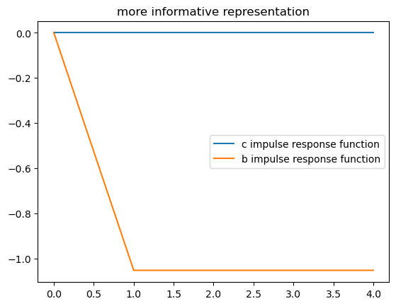
_images/154ffd32a5baafd7b615432a38303fe5bd75d23e98cc5628d66438ffc55cec63.png

The above two impulse response functions show that when the consumer has the information assumed in the more informative representation (5.1), his response to receiving a positive shock of $ε_{t}$ is to leave his consumption unchanged and to save the entire amount of his extra income and then forever roll over the extra bonds that he holds.

To see this notice, that starting from next period on, his debt permanently decreases by $β^{- 1}$

c_res2 / σa, b_res2 / σa

(array([0.0975, 0.0975, 0.0975, 0.0975, 0.0975]),
 array([ 0.  , -0.95, -0.95, -0.95, -0.95]))

plt.title("innovations representation")
plt.plot(range(J), c_res2 / σa, label="c impulse response function")
plt.plot(range(J), b_res2 / σa, label="b impulse response function")
plt.plot([0, J-1], [0, 0], '--', color='k')
plt.legend()

<matplotlib.legend.Legend at 0x7fcb973d8560>

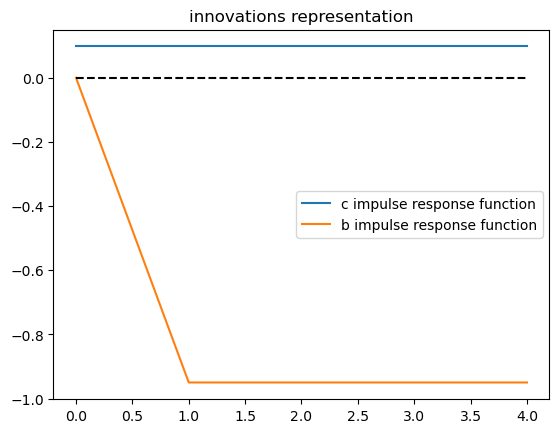
_images/82908cba96f2ec8c493bb562de566e0dbe3953263708e36448b98a04f0209d07.png

The above impulse responses show that when the consumer has only the information that is assumed to be available under the innovations representation (5.2) for ${y_{t} - y_{t - 1}}$ , he responds to a positive $a_{t}$ by permanently increasing his consumption.

He accomplishes this by consuming a fraction $(1 - β^{2})$ of the increment $a_{t}$ to his nonfinancial income and saving the rest, thereby lowering $b_{t + 1}$ in order to finance the permanent increment in his consumption.

The preceding computations confirm what we had derived earlier using paper and pencil.

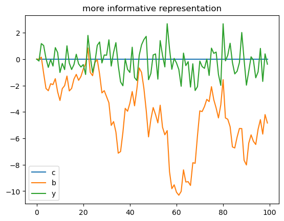
Now let’s simulate some paths of consumption and debt for our two types of consumers while always presenting both types with the same ${y_{t}}$ path.

# Set time length for simulation
T = 100

x1, y1 = LSS1.simulate(ts_length=T)
plt.plot(range(T), y1[0, :], label="c")
plt.plot(range(T), x1[2, :], label="b")
plt.plot(range(T), x1[0, :], label="y")
plt.title("more informative representation")
plt.legend()

<matplotlib.legend.Legend at 0x7fcb4e6d6e40>

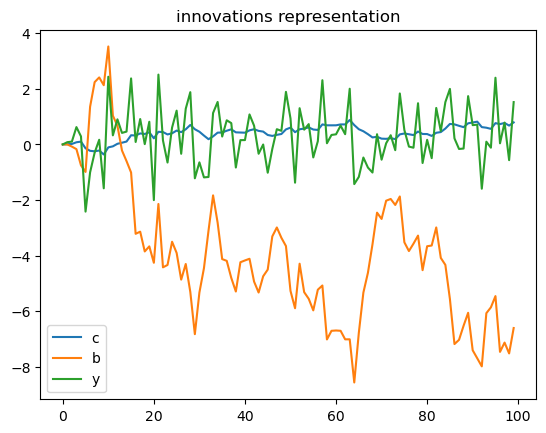
_images/76ef40c08613bba3a09091f8a56258d9bce60ef0f9409a69ff29e7d203b1106f.png

x2, y2 = LSS2.simulate(ts_length=T)
plt.plot(range(T), y2[0, :], label="c")
plt.plot(range(T), x2[2, :], label="b")
plt.plot(range(T), x2[0, :], label="y")
plt.title("innovations representation")
plt.legend()

<matplotlib.legend.Legend at 0x7fcb4dfd96a0>

_images/93b201a60d008f489e8a76a398ab87617994b5d62b8d5f1a02edf0100b91f7d2.png

5.10. Simulating Income Process and Two Associated Shock Processes#

We now form a single ${y_{t}}_{t = 0}^{T}$ realization that we will use to simulate decisions associated with our two types of consumer.

We accomplish this in the following steps.

We form a ${y_{t}, ε_{t}}$ realization by drawing a long simulation of ${ε_{t}}_{t = 0}^{T}$ , where $T$ is a big integer, $ε_{t} = σ_{ε} v_{t}$ , $v_{t}$ is a standard normal scalar, $y_{0} = 100$ , and

$y_{t + 1} - y_{t} = - β^{- 1} ε_{t} + ε_{t + 1} .$
We take the ${y_{t}}$ realization generated in step 1 and form an innovation process ${a_{t}}$ from the formulas

$\begin{aligned} a_{0} & = 0 \\ a_{t} & = \sum_{j = 0}^{t - 1} β^{j} (y_{t - j} - y_{t - j - 1}) + β^{t} a_{0}, t \geq 1 \end{aligned}$
We throw away the first $S$ observations and form a sample ${y_{t}, ε_{t}, a_{t}}_{S + 1}^{T}$ as the realization that we’ll use in the following steps.
We use the step 3 realization to evaluate and simulate the decision rules for $c_{t}, b_{t}$ that Python has computed for us above.

The above steps implement the experiment of comparing decisions made by two consumers having identical incomes at each date but at each date having different information about their future incomes.

5.11. Calculating Innovations in Another Way#

Here we use formula (5.3) above to compute $a_{t + 1}$ as a function of the history $ε_{t + 1}, ε_{t}, ε_{t - 1}, \dots$

Thus, we compute

\begin{array}{r} \begin{aligned} a_{t + 1} & = β a_{t} + ε_{t + 1} - β^{- 1} ε_{t} \\ = β (β a_{t - 1} + ε_{t} - β^{- 1} ε_{t - 1}) + ε_{t + 1} - β^{- 1} ε_{t} \\ = β^{2} a_{t - 1} + β (ε_{t} - β^{- 1} ε_{t - 1}) + ε_{t + 1} - β^{- 1} ε_{t} \\ = ⋮ ⋮ \\ = β^{t + 1} a_{0} + \sum_{j = 0}^{t} β^{j} (ε_{t + 1 - j} - β^{- 1} ε_{t - j}) \\ = β^{t + 1} a_{0} + ε_{t + 1} + (β - β^{- 1}) \sum_{j = 0}^{t - 1} β^{j} ε_{t - j} - β^{t - 1} ε_{0} . \end{aligned} \end{array}

We can verify that we recover the same ${a_{t}}$ sequence computed earlier.

5.12. Another Invertibility Issue#

This quantecon lecture contains another example of a shock-invertibility issue that is endemic to the LQ permanent income or consumption smoothing model.

The technical issue discussed there is ultimately the source of the shock-invertibility issues discussed by Eric Leeper, Todd Walker, and Susan Yang [Leeper et al., 2013] in their analysis of fiscal foresight.