25. Risk and Model Uncertainty#
25.1. Overview#
As an introduction to one possible approach to modeling Knightian uncertainty, this lecture describes static representations of five classes of preferences over risky prospects.
These preference specifications allow us to distinguish risk from uncertainty along lines proposed by [Knight, 1921].
All five preference specifications incorporate risk aversion, meaning displeasure from risks governed by well known probability distributions.
Two of them also incorporate uncertainty aversion, meaning dislike of not knowing a probability distribution.
The preference orderings are
Expected utility preferences
Constraint preferences
Multiplier preferences
Risk-sensitive preferences
Ex post Bayesian expected utility preferences
This labeling scheme is taken from [Hansen and Sargent, 2001].
Constraint and multiplier preferences express aversion to not knowing a unique probability distribution that describes random outcomes.
Expected utility, risk-sensitive, and ex post Bayesian expected utility preferences all attribute a unique known probability distribution to a decision maker.
We present things in a simple before-and-after one-period setting.
In addition to learning about these preference orderings, this lecture also describes some interesting code for computing and graphing some representations of indifference curves, utility functions, and related objects.
Staring at these indifference curves provides insights into the different preferences.
Watch for the presence of a kink at the
We begin with some that we’ll use to create some graphs.
# Package imports
import numpy as np
import matplotlib as mpl
import matplotlib.pyplot as plt
from matplotlib import rc, cm
from mpl_toolkits.mplot3d import Axes3D
from scipy import optimize, stats
from scipy.io import loadmat
from matplotlib.collections import LineCollection
from matplotlib.colors import ListedColormap, BoundaryNorm
from numba import njit
25.2. Basic objects#
Basic ingredients are
a set of states of the world
plans describing outcomes as functions of the state of the world,
a utility function mapping outcomes into utilities
either a probability distribution or a set of probability distributions over states of the world; and
a way of measuring a discrepancy between two probability distributions.
In more detail, we’ll work with the following setting.
A finite set of possible states
A (consumption) plan is a function
Relative entropy
or
Remark: A likelihood ratio
where
Evidently,
and relative entropy is
In the three figures below, we plot relative entropy from several perspectives.
Our first figure depicts entropy as a function of
When
However, when
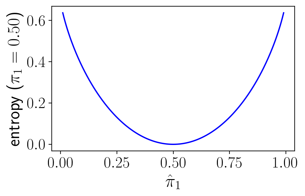
Fig. 25.1 Figure 1#
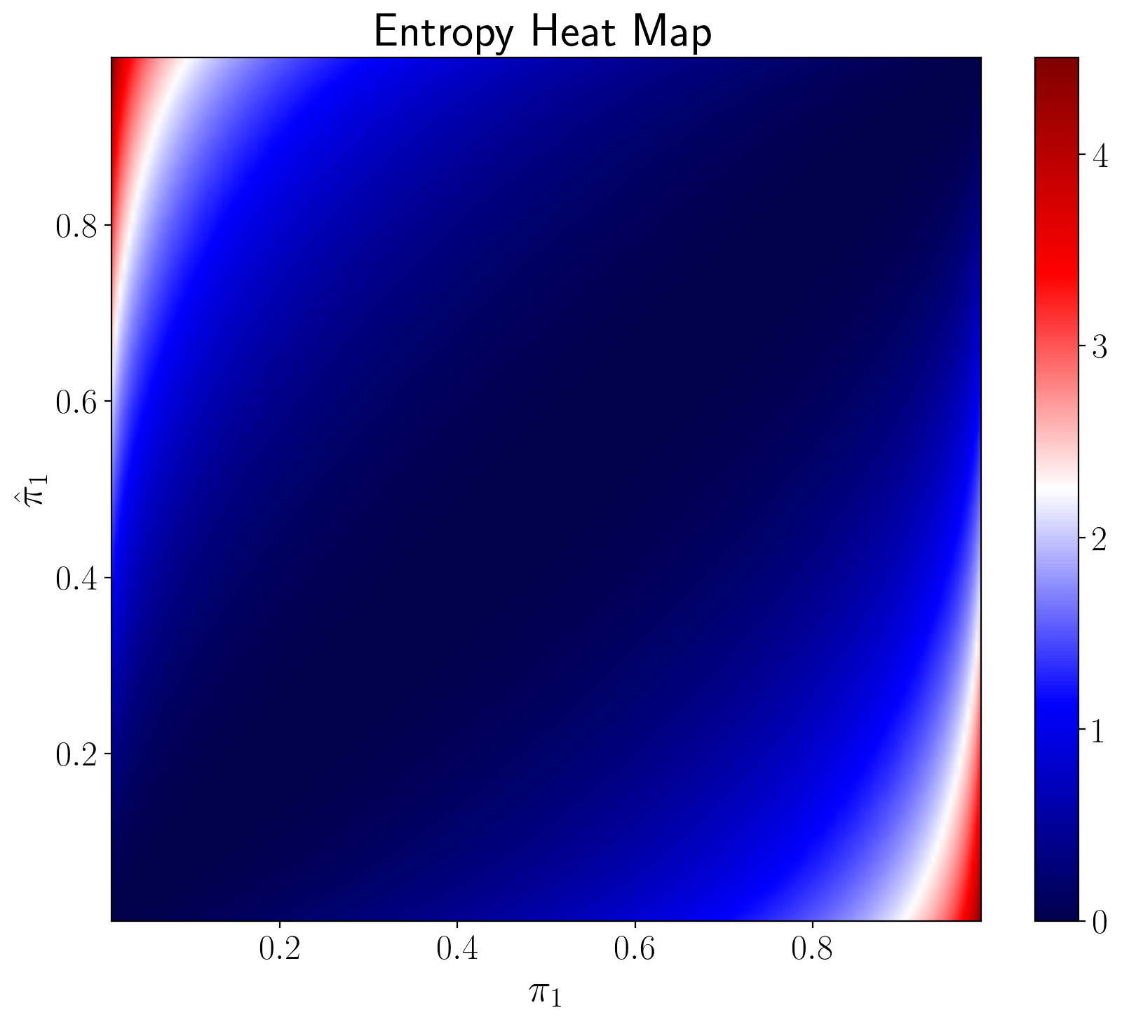
The heat maps in the next two figures vary both
The following figure plots entropy.
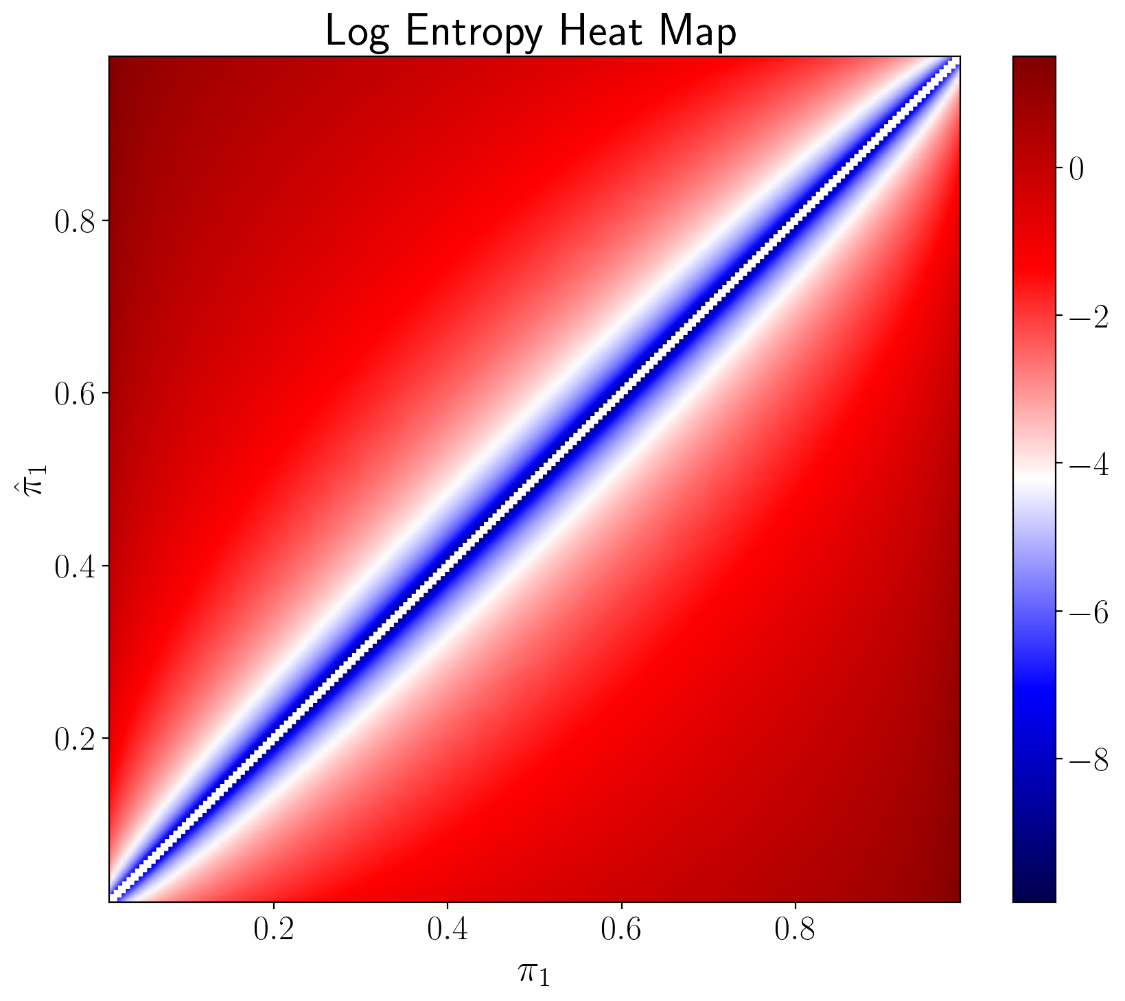
The next figure plots the logarithm of entropy.
3.8205752275831846
/tmp/ipykernel_7948/3759713737.py:2: RuntimeWarning: divide by zero encountered in log
  plt.pcolormesh(x, y, np.log(ent_vals_mat.T), shading='gouraud', cmap='seismic')
25.3. Five preference specifications#
We describe five types of preferences over plans.
Expected utility preferences
Constraint preferences
Multiplier preferences
Risk-sensitive preferences
Ex post Bayesian expected utility preferences
Expected utility, risk-sensitive, and ex post Bayesian prefernces are each cast in terms of a unique probability distribution, so they can express risk-aversion, but not model ambiguity aversion.
Multiplier and constraint prefernces both express aversion to concerns about model misppecification, i.e., model uncertainty; both are cast in terms of a set or sets of probability distributions.
The set of distributions expresses the decision maker’s ambiguity about the probability model.
Minimization over probability distributions expresses his aversion to ambiguity.
25.4. Expected utility#
A decision maker is said to have expected utility preferences when he ranks plans
where
A known
Curvature of
25.5. Constraint preferences#
A decision maker is said to have constraint preferences when he ranks plans
subject to
and
In (25.3),
As noted earlier,
Larger values of the entropy constraint
Following [Hansen and Sargent, 2001] and [Hansen and Sargent, 2008], we call minimization problem (25.2) subject to (25.3) and(25.4) a constraint problem.
To find minimizing probabilities, we form a Lagrangian
where
Subject to the additional constraint that
The minimizing probability distortions (likelihood ratios) are
To compute the Lagrange multiplier
or
for
For a fixed
With
The indirect (expected) utility function under constraint preferences is
Entropy evaluated at the minimizing probability distortion
(25.6) equals
Expression (25.9) implies that
where the last term is
25.6. Multiplier preferences#
A decision maker is said to have multiplier preferences when he ranks consumption plans
where minimization is subject to
Here
Lower values of the penalty parameter
Following [Hansen and Sargent, 2001] and [Hansen and Sargent, 2008], we call the minimization problem on the right side of (25.11) a multiplier problem.
The minimizing probability distortion that solves the multiplier problem is
We can solve
to find an entropy level
For a fixed
The forms of expressions (25.6) and (25.12) are identical, but the Lagrange multiplier
Formulas (25.6) and (25.12) show that worst-case probabilities are context specific in the sense that they depend on both the utility function
If we add
25.7. Risk-sensitive preferences#
Substituting
Here
It defines a risk-sensitive preference ordering over plans
Because it is not linear in utilities
Because risk-sensitive preferences use a unique probability distribution, they apparently express no model distrust or ambiguity.
Instead, they make an additional adjustment for risk-aversion beyond that embedded in the curvature of
For
For large values of
Under expected utility, i.e.,
The two panels in the next figure below can help us to visualize the extra adjustment for risk that the risk-sensitive operator entails.
This will help us understand how the
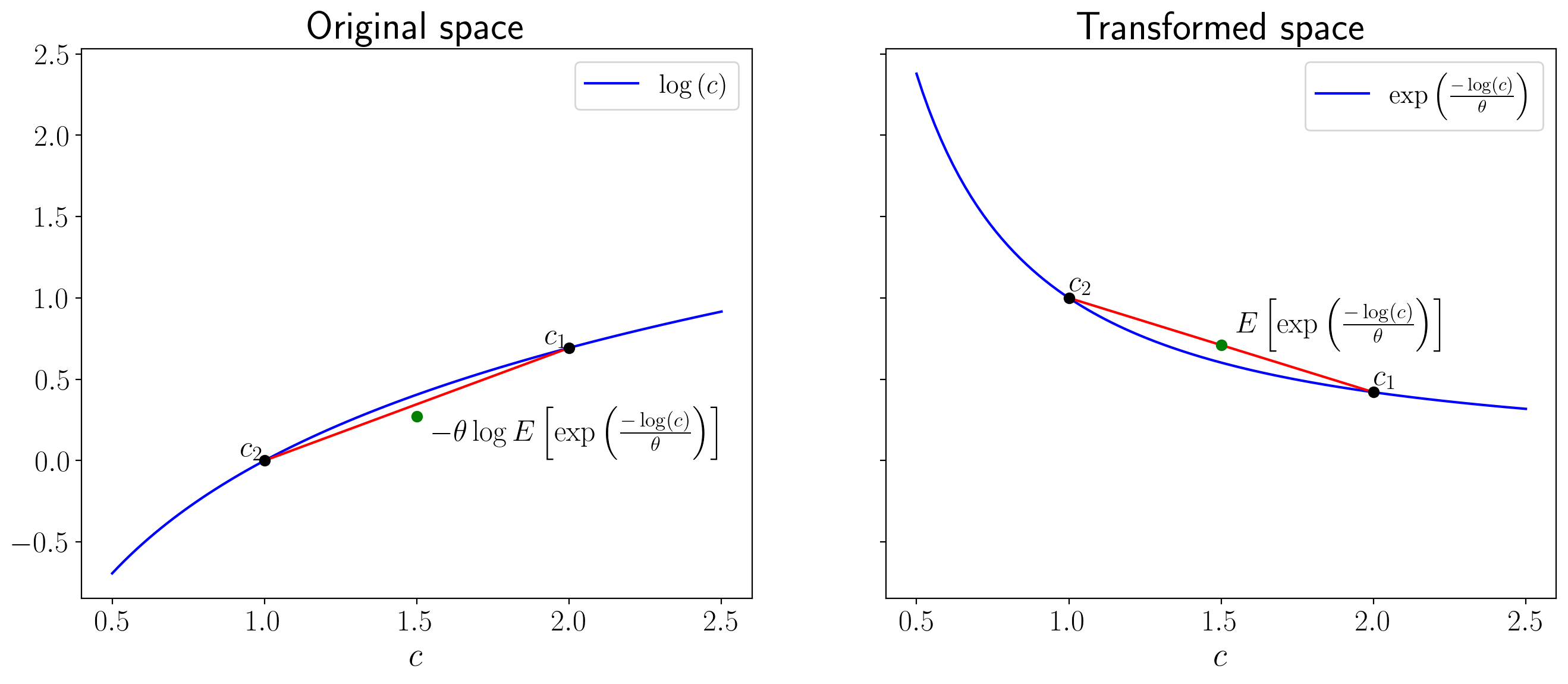
The panel on the right portrays how the transformation
In the left panel, the red line is our tool for computing the mathematical expectation for different
values of
The green lot indicates the mathematical expectation of
Notice that the distance between the green dot and the curve is greater in the transformed space than the original space as a result of additional curvature.
The inverse transformation
The gap between the green dot and the red line on the left panel measures the additional adjustment for risk that risk-sensitive preferences make relative to plain vanilla expected utility preferences.
25.7.1. Digression on moment generating functions#
The risk-sensitivity operator
In particular, a principal constinuent of the
is evidently a moment generating function for the random variable
is a cumulant generating function,
where
Then
In general, when
These statements extend to cases with continuous probability distributions for
For the special case
which becomes expected utility
The right side of equation (25.16) is a special case of stochastic differential utility preferences in which consumption plans are ranked not just by their expected utilities
25.8. Ex post Bayesian preferences#
A decision maker is said to have ex post Bayesian preferences when he ranks consumption plans according to the expected utility function
where
At
25.9. Comparing preferences#
For the special case in which
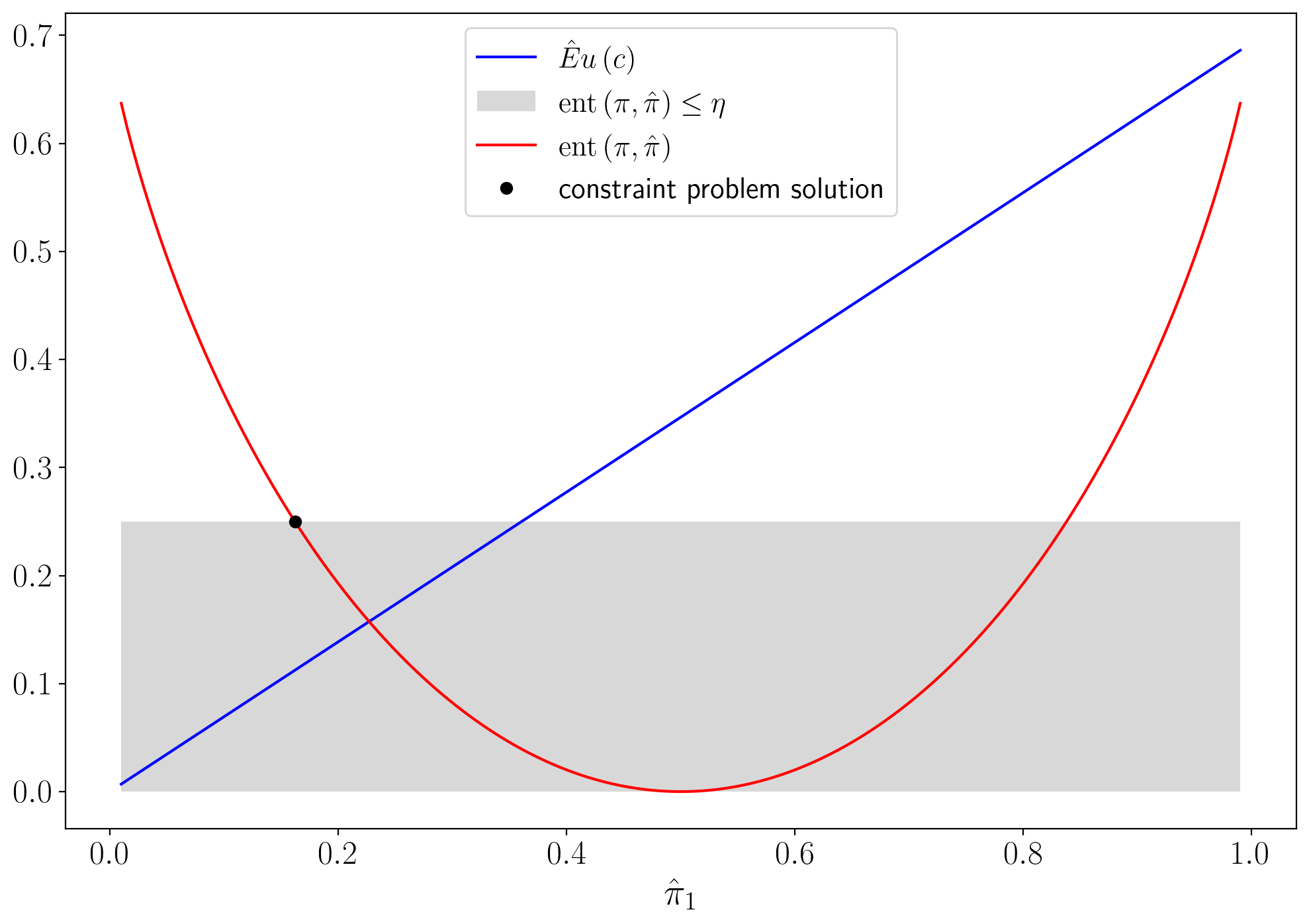
The first figure graphs entropy as a function of
It also plots expected utility under the twisted probability distribution, namely,
The entropy constraint
Unless
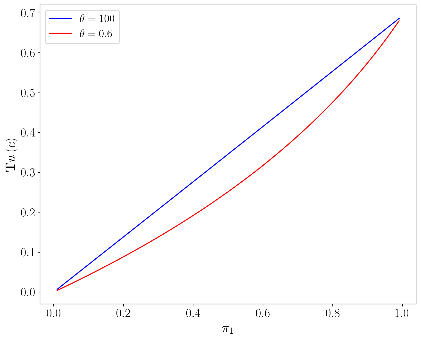
The next figure shows the function
The argument of the function is
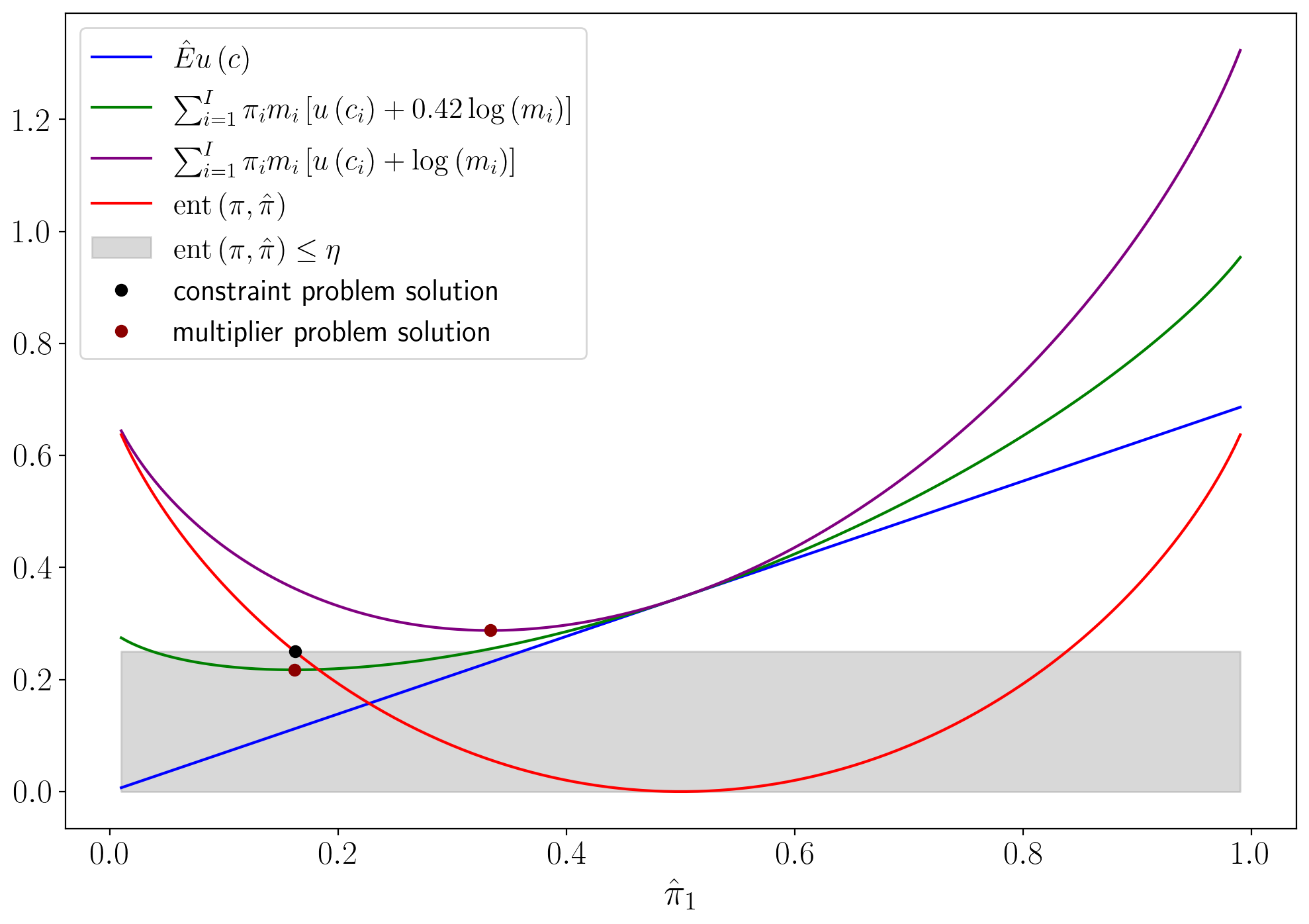
Evidently, from this figure and also from formula (25.12), lower values of
The figure
indicates how one can construct a Lagrange multiplier
Thus, to draw the figure, we set the penalty parameter for
multiplier preferences
The penalty parameter
25.10. Risk aversion and misspecification aversion#
All five types of preferences use curvature of
Constraint preferences express concern about misspecification or ambiguity for short with a positive
Multiplier preferences express misspecification concerns with a parameter
By penalizing minimization over the
likelihood ratio
Formulas (25.6) assert that the decision maker acts as if
he is pessimistic relative to an approximating model
It expresses what [Bucklew, 2004] [p. 27] calls a statistical version of Murphy’s law:
The minimizing likelihood ratio
As expressed by the value function bound (25.19) to be displayed below, the decision maker uses pessimism instrumentally to protect himself against model misspecification.
The penalty parameter
A decision rule is said to be undominated in the sense of Bayesian
decision theory if there exists a probability distribution
A decision rule is said to be admissible if it is undominated.
[Hansen and Sargent, 2008] use ex post Bayesian preferences to show that robust decision rules are undominated and therefore admissible.
25.11. Indifference curves#
Indifference curves illuminate how concerns about robustness affect
asset pricing and utility costs of fluctuations. For
Expected utility:
Constraint and ex post Bayesian preferences:
where
Multiplier and risk-sensitive preferences:
When
As we shall see soon when we discuss state price deflators, this gives rise to higher estimates of prices of risk.
For an example with
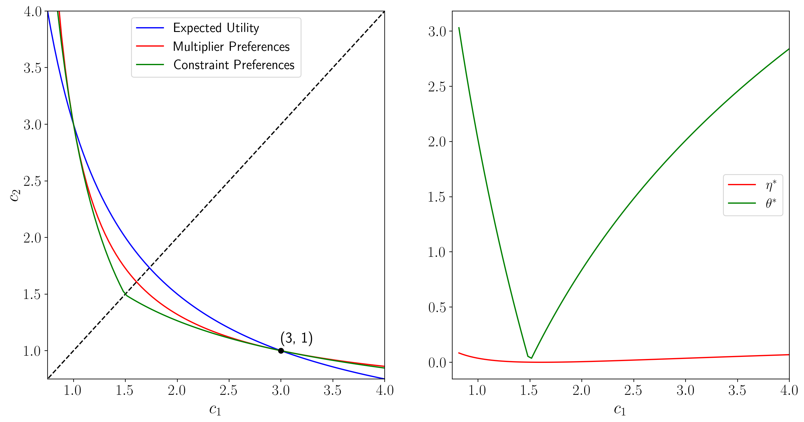
The following figure shows indifference curves going through a point along the 45 degree line.
Kink at 45 degree line
Notice the kink in the indifference curve for constraint preferences at the 45 degree line.
To understand the source of the kink, consider how the Lagrange multiplier and worst-case probabilities vary with the consumption plan under constraint preferences.
For fixed
This pattern makes the Lagrange multiplier
The discontinuity in the worst case
The code for generating the preceding figure is somewhat intricate we formulate a root finding problem for finding indifference curves.
Here is a brief literary description of the method we use.
Parameters
Consumption bundle
Penalty parameter
Utility function
Probability vector
Algorithm:
Compute
Given values for
Expected utility:
Multiplier preferences: solve
Constraint preference: solve
Remark: It seems that the constraint problem is hard to solve in its original form, i.e. by finding the distorting measure that minimizes the expected utility.
It seems that viewing equation (25.7) as a root finding problem works much better.
But notice that equation (25.7) does not always have a solution.
Under
Conjecture: when our numerical method fails it because the derivative of the objective doesn’t exist for our choice of parameters.
Remark: It is tricky to get the algorithm to work properly for all values of
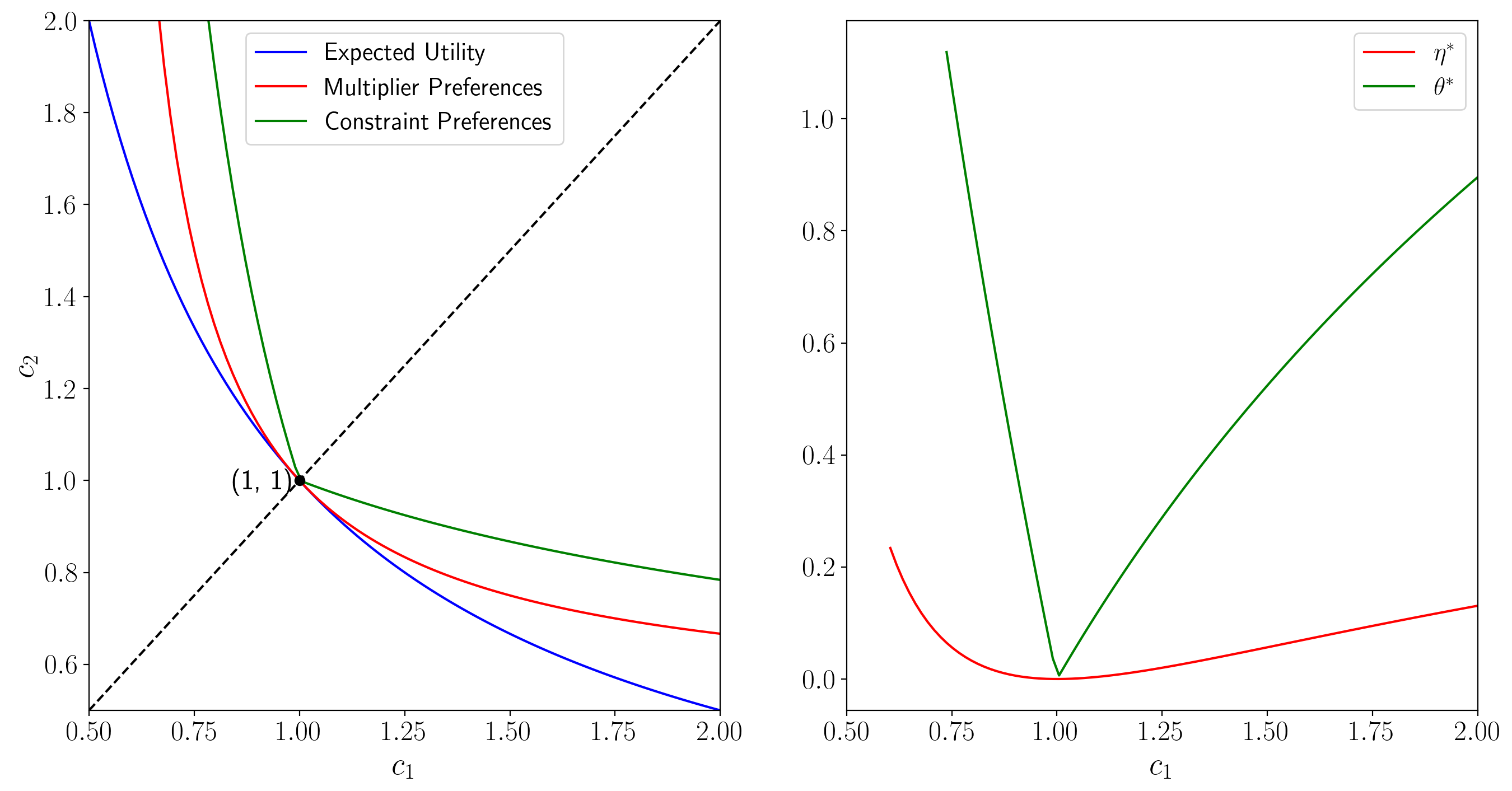
Tangent indifference curves off 45 degree line
For a given
The following figure shows indifference curves for
multiplier and constraint preferences through a point off the 45 degree
line, namely,
Note that all three lines of the left graph intersect at (1, 3). While the intersection at (3, 1) is hard-coded, the intersection at (1,3) arises from the computation, which confirms that the code seems to be working properly.
As we move along the (kinked) indifference curve for the constraint
preferences for a given
As we move along the (smooth) indifference curve for the
multiplier preferences for a given penalty parameter
For constraint preferences, there is a kink in the indifference curve.
For ex post Bayesian preferences, there are effectively two sets of indifference curves depending on which
side of the 45 degree line the
There are two sets of indifference curves because, while the worst-case probabilities differ above and below the 45 degree line, the idea of ex post Bayesian preferences is to use a single probability distribution to compute expected utilities for all consumption bundles.
Indifference curves through point
25.12. State price deflators#
Concerns about model uncertainty boost prices of risk that are embedded
in state-price deflators. With complete markets, let
The budget set of a representative consumer
having endowment
When a representative consumer has multiplier preferences, the state prices are
The worst-case likelihood ratio
State prices agree under multiplier and constraint preferences when
The next figure can help us think about state-price deflators under our different preference orderings.
In this figure, budget line and indifference curves through point
Figure 2.7:
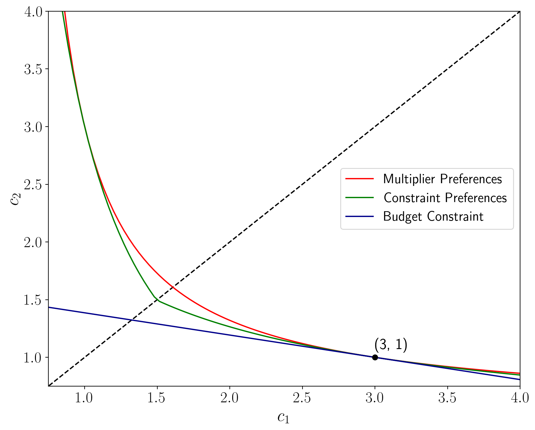
Because budget constraints are linear, asset prices are identical under
multiplier and constraint preferences for which
However, as we note next, though they are tangent at the endowment point, the fact that indifference curves differ for multiplier and constraint preferences means that certainty equivalent consumption compensations of the kind that [Lucas, 1987], [Hansen et al., 1999], [Tallarini, 2000], and [Barillas et al., 2009] used to measure the costs of business cycles must differ.
25.12.1. Consumption-equivalent measures of uncertainty aversion#
For each of our five types of preferences, the following figure allows us to construct a certainty
equivalent point
Figure 2.8:
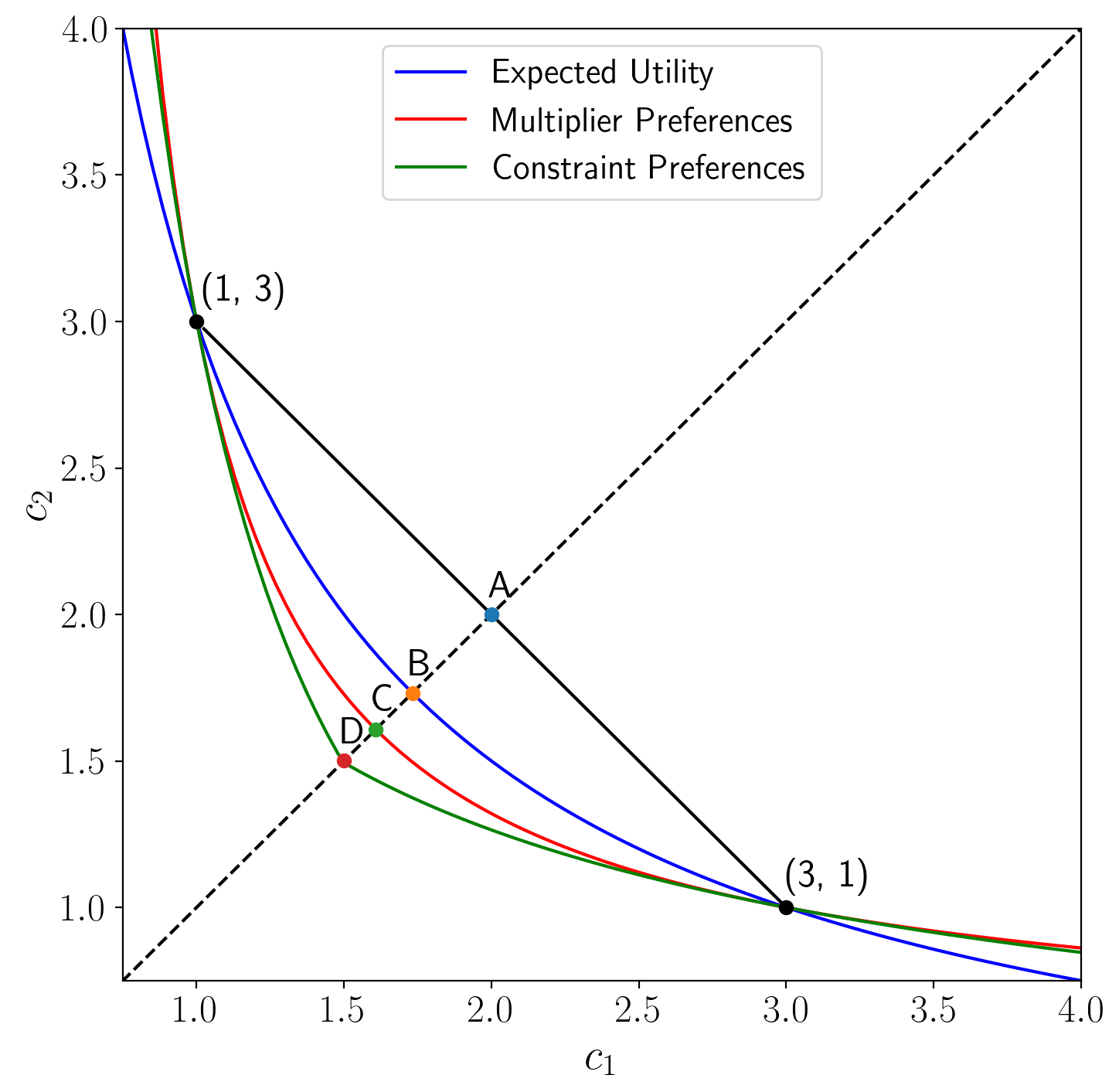
The figure indicates that the certainty equivalent
level
The gap between these certainty equivalents measures the uncertainty aversion of the multiplier preferences or constraint preferences consumer.
The gap between the expected value
The gap between points
The gap between points B and D measures the constraint preference consumer’s aversion to model uncertainty.
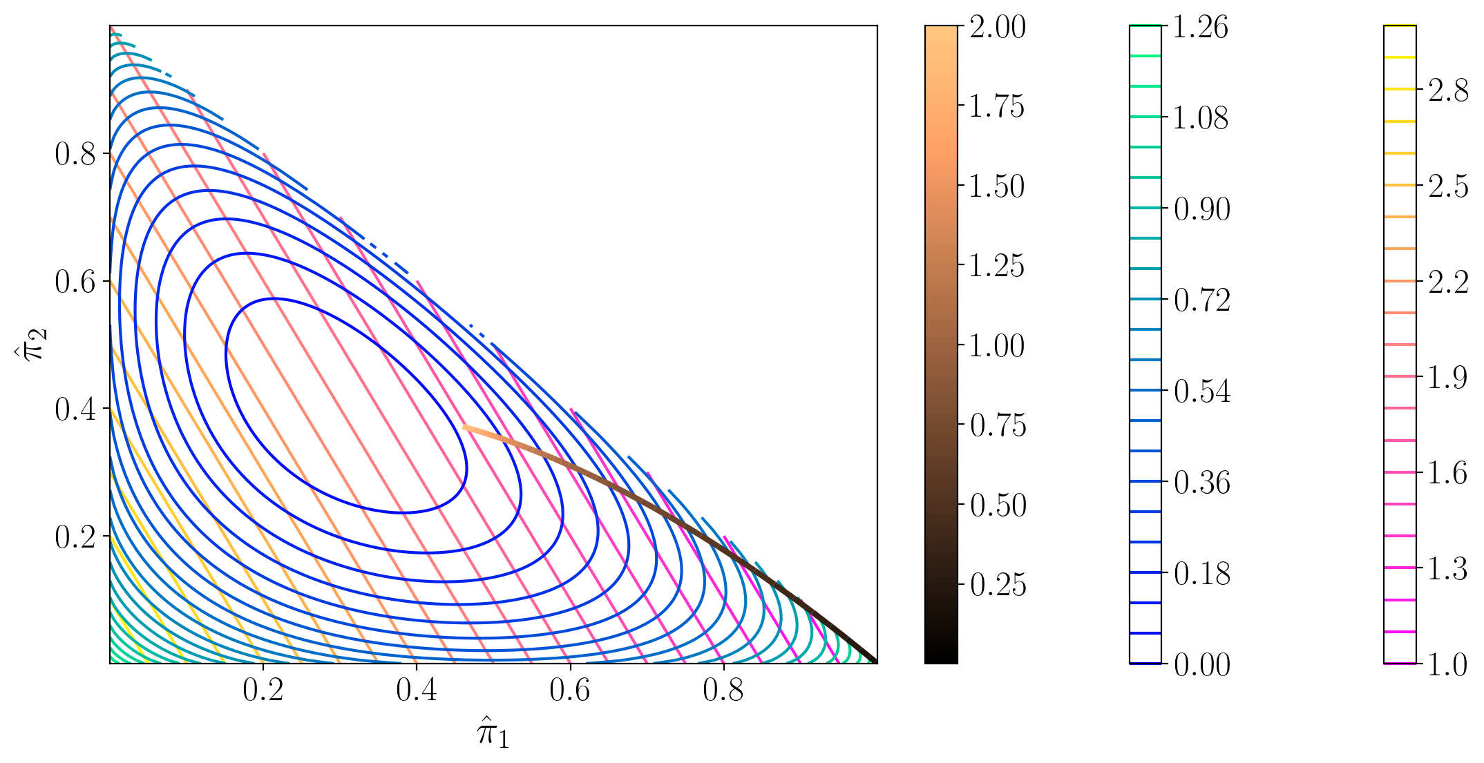
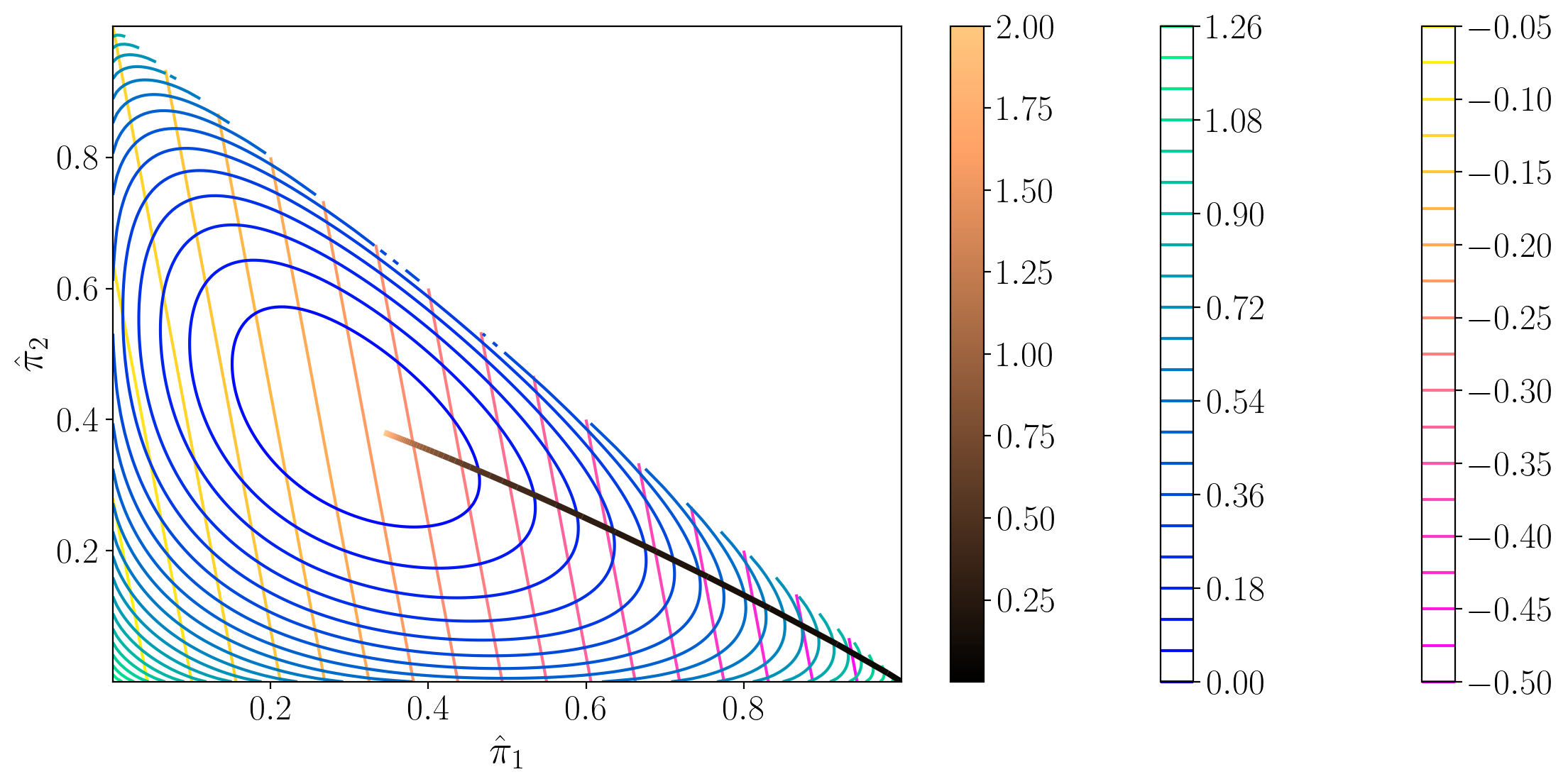
25.13. Iso-utility and iso-entropy curves and expansion paths#
The following figures show iso-entropy and iso-utility lines for the special case in which
The iso-utility lines are the level curves of
and are linear in
This is what it means to say ‘expected utility is linear in probabilities.’
Both figures plot the locus of points of tangency between the iso-entropy and the iso-utility
curves that is traced out as one varies
While the iso-entropy lines are identical in the two figures, these ‘expansion paths’ differ because the utility functions differ,
meaning that for a given
Color bars:
First color bar: variation in
Second color bar: variation in utility levels
Third color bar: variation in entropy levels
/tmp/ipykernel_7948/3904427642.py:36: RuntimeWarning: invalid value encountered in divide
  m =  m_unnormalized / (π * m_unnormalized).sum()
/tmp/ipykernel_7948/3904427642.py:35: RuntimeWarning: overflow encountered in exp
  m_unnormalized = np.exp(-u(c) / θ)
/tmp/ipykernel_7948/3904427642.py:36: RuntimeWarning: invalid value encountered in divide
  m =  m_unnormalized / (π * m_unnormalized).sum()
25.14. Bounds on expected utility#
Suppose that a decision maker wants a lower bound on expected utility
An attractive feature of multiplier and constraint preferences is that they carry with them such a bound.
To show this, it is useful to collect some findings in the following string of inequalities associated with multiplier preferences:
where
The inequality in the last line just asserts that minimizers minimize.
Therefore, we have the following useful bound:
The left side is expected utility under the probability distribution
The right side is a lower bound on expected utility
under all distributions expressed as an affine function of relative
entropy
The bound is attained for
The intercept in the bound is the risk-sensitive criterion
Lowering
it lowers the intercept
it lowers the absolute value of the slope, which makes the bound more informative for larger values of relative entropy
The following figure reports best-case and worst-case expected utilities.
We calculate the lines in this figure numerically by solving optimization problems with respect to the change of measure.
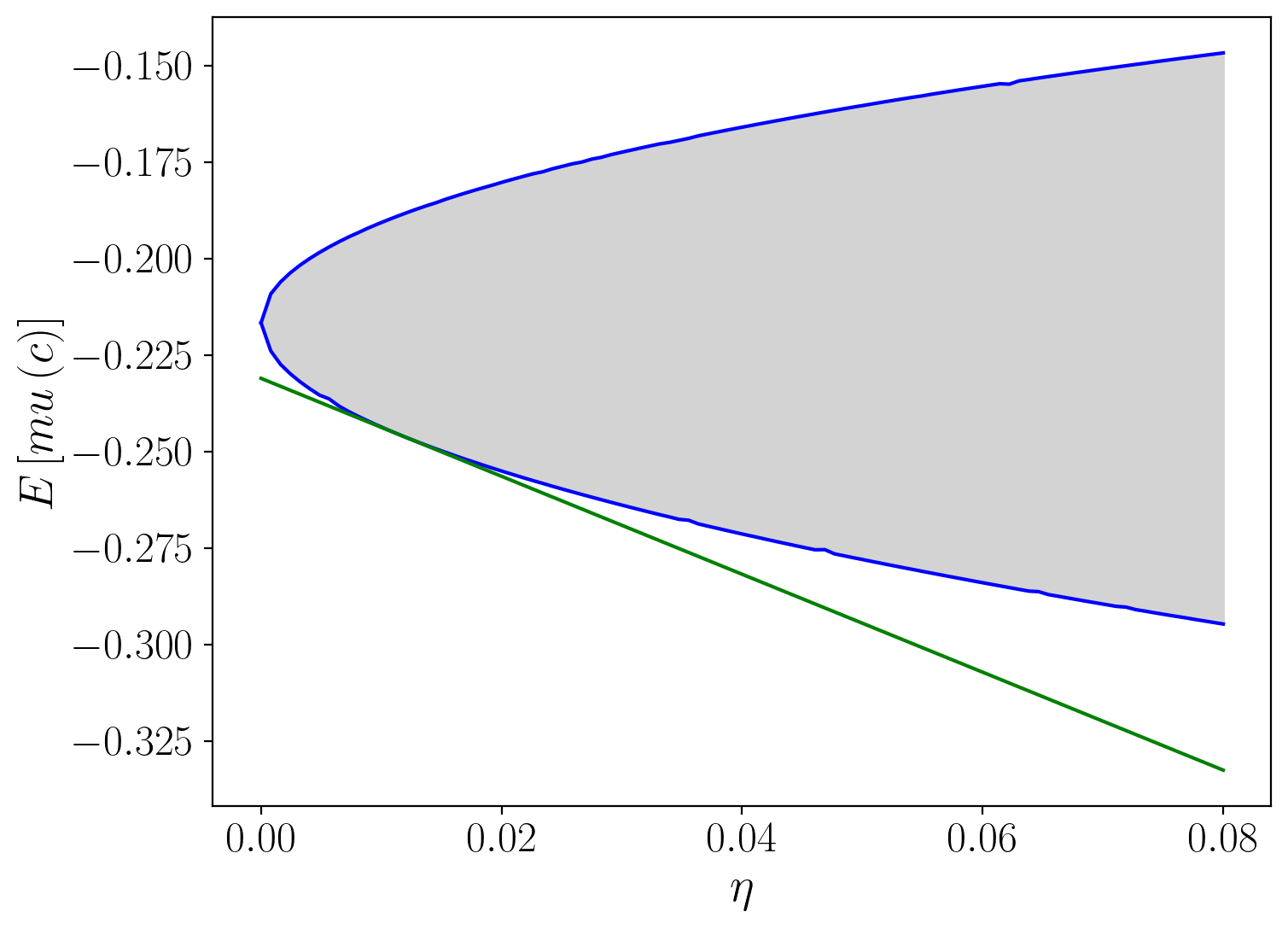
In this figure, expected utility is on the co-ordinate axis while entropy is on the ordinate axis.
The lower curved line depicts
expected utility under the worst-case model associated with each value
of entropy
The higher curved line depicts expected utility under the best-case
model indexed by the value of the Lagrange multiplier
(Here
Points between these two curves are
possible values of expected utility for some distribution with entropy
less than or equal to the value
The straight line depicts the right side of inequality (25.19) for a particular value of the penalty parameter
As noted, when one lowers
Thus, as
However, as
The slope of straight line depicting a bound is
This is an application of the envelope theorem.
25.15. Why entropy?#
Beyond the helpful mathematical fact that it leads directly to convenient exponential twisting formulas (25.6) and (25.12) for worst-case probability distortions, there are two related justifications for using entropy to measure discrepancies between probability distribution.
One arises from the role of entropy in statistical tests for discriminating between models.
The other comes from axioms.
25.15.1. Entropy and statistical detection#
Robust control theory starts with a decision maker who has constructed a good baseline approximating model whose free parameters he has estimated to fit historical data well.
The decision maker recognizes that actual outcomes might be generated by one of a vast number of other models that fit the historical data nearly as well as his.
Therefore, he wants to evaluate outcomes under a set of alternative models that are plausible in the sense of being statistically close to his model.
He uses relative entropy to quantify what close means.
[Anderson et al., 2003] and [Barillas et al., 2009]describe links between entropy and large deviations
bounds on test statistics for discriminating between models, in particular, statistics that describe the probability of making an error in applying a likelihood ratio test to decide whether model A or model B
generated a data record of length
For a given sample size, an
informative bound on the detection error probability is a function of
the entropy parameter
[Anderson et al., 2003] and [Hansen and Sargent, 2008] also
use detection error probabilities to calibrate reasonable values of the
penalty parameter
For a fixed sample size and a fixed
They then invert this function to calibrate
To indicate outcomes from this approach, the following figure plots the histogram for U.S. quarterly consumption growth along with a representative agent’s approximating density and a worst-case density that [Barillas et al., 2009] show imply high measured market prices of risk even when a representative consumer has the unit coefficient of relative risk aversion associated with a logarithmic one-period utility function.
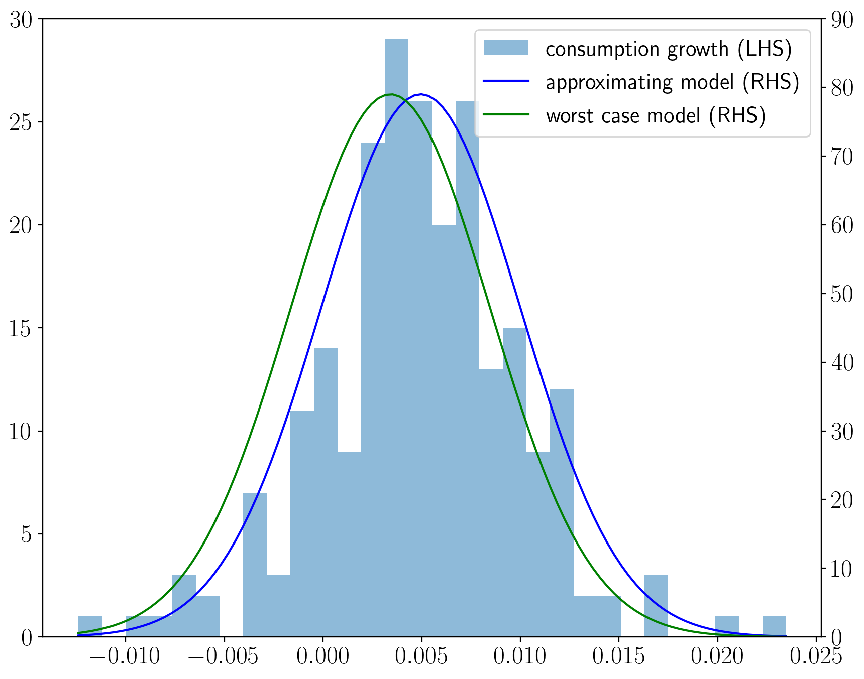
The density for the approximating model is
The consumer’s value function under logarithmic utility implies that the worst-case model is
The worst-case model appears to fit the histogram nearly as well as the approximating model.
25.15.2. Axiomatic justifications#
Multiplier and constraint preferences are both special cases of what [Maccheroni et al., 2006] call variational preferences.
They provide an axiomatic foundation for variational preferences and describe how they express ambiguity aversion.
Constraint preferences are particular instances of the multiple priors model of [Gilboa and Schmeidler, 1989].