8. Markov Jump Linear Quadratic Dynamic Programming#

In addition to what’s in Anaconda, this lecture will need the following libraries:

!pip install --upgrade quantecon

8.1. Overview#

This lecture describes Markov jump linear quadratic dynamic programming, an extension of the method described in the first LQ control lecture.

Markov jump linear quadratic dynamic programming is described and analyzed in [Do Val et al., 1999] and the references cited there.

The method has been applied to problems in macroeconomics and monetary economics by [Svensson et al., 2008] and [Svensson and Williams, 2009].

The periodic models of seasonality described in chapter 14 of [Hansen and Sargent, 2013] are a special case of Markov jump linear quadratic problems.

Markov jump linear quadratic dynamic programming combines advantages of

the computational simplicity of linear quadratic dynamic programming, with
the ability of finite state Markov chains to represent interesting patterns of random variation.

The idea is to replace the constant matrices that define a linear quadratic dynamic programming problem with $N$ sets of matrices that are fixed functions of the state of an $N$ state Markov chain.

The state of the Markov chain together with the continuous $n \times 1$ state vector $x_{t}$ form the state of the system.

For the class of infinite horizon problems being studied in this lecture, we obtain $N$ interrelated matrix Riccati equations that determine $N$ optimal value functions and $N$ linear decision rules.

One of these value functions and one of these decision rules apply in each of the $N$ Markov states.

That is, when the Markov state is in state $j$ , the value function and the decision rule for state $j$ prevails.

8.2. Review of useful LQ dynamic programming formulas#

To begin, it is handy to have the following reminder in mind.

A linear quadratic dynamic programming problem consists of a scalar discount factor $β \in (0, 1)$ , an $n \times 1$ state vector $x_{t}$ , an initial condition for $x_{0}$ , a $k \times 1$ control vector $u_{t}$ , a $p \times 1$ random shock vector $w_{t + 1}$ and the following two triples of matrices:

A triple of matrices $(R, Q, W)$ defining a loss function

r (x_{t}, u_{t}) = x_{t}^{'} R x_{t} + u_{t}^{'} Q u_{t} + 2 u_{t}^{'} W x_{t}

a triple of matrices $(A, B, C)$ defining a state-transition law

x_{t + 1} = A x_{t} + B u_{t} + C w_{t + 1}

The problem is

- x_{0}^{'} P x_{0} - ρ = min_{{u_{t}}_{t = 0}^{\infty}} E \sum_{t = 0}^{\infty} β^{t} r (x_{t}, u_{t})

subject to the transition law for the state.

The optimal decision rule has the form

u_{t} = - F x_{t}

and the optimal value function is of the form

- (x_{t}^{'} P x_{t} + ρ)

where $P$ solves the algebraic matrix Riccati equation

P = R + β A^{'} P A - (β B^{'} P A + W)^{'} (Q + β B P B)^{- 1} (β B P A + W)

and the constant $ρ$ satisfies

ρ = β (ρ + t r a c e (P C C^{'}))

and the matrix $F$ in the decision rule for $u_{t}$ satisfies

F = (Q + β B^{'} P B)^{- 1} (β (B^{'} P A) + W)

With the preceding formulas in mind, we are ready to approach Markov Jump linear quadratic dynamic programming.

8.3. Linked Riccati equations for Markov LQ dynamic programming#

The key idea is to make the matrices $A, B, C, R, Q, W$ fixed functions of a finite state $s$ that is governed by an $N$ state Markov chain.

This makes decision rules depend on the Markov state, and so fluctuate through time in limited ways.

In particular, we use the following extension of a discrete-time linear quadratic dynamic programming problem.

We let $s_{t} \in [1, 2, \dots, N]$ be a time $t$ realization of an $N$ -state Markov chain with transition matrix $Π$ having typical element $Π_{i j}$ .

Here $i$ denotes today and $j$ denotes tomorrow and

Π_{i j} = P r o b (s_{t + 1} = j | s_{t} = i)

We’ll switch between labeling today’s state as $s_{t}$ and $i$ and between labeling tomorrow’s state as $s_{t + 1}$ or $j$ .

The decision-maker solves the minimization problem:

min_{{u_{t}}_{t = 0}^{\infty}} E \sum_{t = 0}^{\infty} β^{t} r (x_{t}, s_{t}, u_{t})

with

r (x_{t}, s_{t}, u_{t}) = x_{t}^{'} R_{s_{t}} x_{t} + u_{t}^{'} Q_{s_{t}} u_{t} + 2 u_{t}^{'} W_{s_{t}} x_{t}

subject to linear laws of motion with matrices $(A, B, C)$ each possibly dependent on the Markov-state- $s_{t}$ :

x_{t + 1} = A_{s_{t}} x_{t} + B_{s_{t}} u_{t} + C_{s_{t}} w_{t + 1}

where ${w_{t + 1}}$ is an i.i.d. stochastic process with $w_{t + 1} \sim N (0, I)$ .

The optimal decision rule for this problem has the form

u_{t} = - F_{s_{t}} x_{t}

and the optimal value functions are of the form

- (x_{t}^{'} P_{s_{t}} x_{t} + ρ_{s_{t}})

or equivalently

- x_{t}^{'} P_{i} x_{t} - ρ_{i}

The optimal value functions $- x^{'} P_{i} x - ρ_{i}$ for $i = 1, \dots, n$ satisfy the $N$ interrelated Bellman equations

\begin{aligned} - x^{'} P_{i} x - ρ_{i} & = max_{u} - x^{'} R_{i} x & + u^{'} Q_{i} u + 2 u^{'} W_{i} x + β \sum_{j} Π_{i j} E ((A_{i} x + B_{i} u + C_{i} w)^{'} P_{j} (A_{i} x + B_{i} u + C_{i} w) x + ρ_{j}) \end{aligned}

The matrices $P_{s_{t}} = P_{i}$ and the scalars $ρ_{s_{t}} = ρ_{i}, i = 1, \dots$ , n satisfy the following stacked system of algebraic matrix Riccati equations:

P_{i} = R_{i} + β \sum_{j} A_{i}^{'} P_{j} A_{i} Π_{i j} - \sum_{j} Π_{i j} [(β B_{i}^{'} P_{j} A_{i} + W_{i})^{'} (Q + β B_{i}^{'} P_{j} B_{i})^{- 1} (β B_{i}^{'} P_{j} A_{i} + W_{i})]

ρ_{i} = β \sum_{j} Π_{i j} (ρ_{j} + t r a c e (P_{j} C_{i} C_{i}^{'}))

and the $F_{i}$ matrices in the optimal decision rules are

F_{i} = (Q_{i} + β \sum_{j} Π_{i j} B_{i}^{'} P_{j} B_{i})^{- 1} (β \sum_{j} Π_{i j} (B_{i}^{'} P_{j} A_{i}) + W_{i})

8.4. Applications#

We now describe Python code and some examples.

To begin, we import these Python modules

import numpy as np
import quantecon as qe
import matplotlib.pyplot as plt
from mpl_toolkits.mplot3d import Axes3D

# Set discount factor
β = 0.95

8.5. Example 1#

This example is a version of a classic problem of optimally adjusting a variable $k_{t}$ to a target level in the face of costly adjustment.

This provides a model of gradual adjustment.

Given $k_{0}$ , the objective function is

max_{{k_{t}}_{t = 1}^{\infty}} E_{0} \sum_{t = 0}^{\infty} β^{t} r (s_{t}, k_{t})

where the one-period payoff function is

r (s_{t}, k_{t}) = f_{1, s_{t}} k_{t} - f_{2, s_{t}} k_{t}^{2} - d_{s_{t}} (k_{t + 1} - k_{t})^{2},

$E_{0}$ is a mathematical expectation conditioned on time $0$ information $x_{0}, s_{0}$ and the transition law for continuous state variable $k_{t}$ is

k_{t + 1} - k_{t} = u_{t}

We can think of $k_{t}$ as the decision-maker’s capital and $u_{t}$ as costs of adjusting the level of capital.

We assume that $f_{1} (s_{t}) > 0$ , $f_{2} (s_{t}) > 0$ , and $d (s_{t}) > 0$ .

Denote the state transition matrix for Markov state $s_{t} \in {1, 2}$ as $Π$ :

Pr (s_{t + 1} = j ∣ s_{t} = i) = Π_{i j}

Let $x_{t} = [\begin{matrix} k_{t} \\ 1 \end{matrix}]$

We can represent the one-period payoff function $r (s_{t}, k_{t})$ as

\begin{array}{r} \begin{matrix} r (s_{t}, k_{t}) = f_{1, s_{t}} k_{t} - f_{2, s_{t}} k_{t}^{2} - d_{s_{t}} u_{t}^{2} \\ = - x_{t}^{'} \underset{\equiv R (s_{t})}{\underset{⏟}{[\begin{array}{c} f_{2, s_{t}} & - \frac{f_{1, s_{t}}}{2} \\ - \frac{f_{1, s_{t}}}{2} & 0 \end{array}]}} x_{t} + \underset{\equiv Q (s_{t})}{\underset{⏟}{d_{s_{t}}}} u_{t}^{2} \end{matrix} \end{array}

and the state-transition law as

\begin{array}{r} x_{t + 1} = [\begin{array}{c} k_{t + 1} \\ 1 \end{array}] = \underset{\equiv A (s_{t})}{\underset{⏟}{I_{2}}} x_{t} + \underset{\equiv B (s_{t})}{\underset{⏟}{[\begin{array}{c} 1 \\ 0 \end{array}]}} u_{t} \end{array}

def construct_arrays1(f1_vals=[1. ,1.],
                      f2_vals=[1., 1.],
                      d_vals=[1., 1.]):
    """
    Construct matrices that map the problem described in example 1
    into a Markov jump linear quadratic dynamic programming problem
    """

    # Number of Markov states
    m = len(f1_vals)
    # Number of state and control variables
    n, k = 2, 1

    # Construct sets of matrices for each state
    As = [np.eye(n) for i in range(m)]
    Bs = [np.array([[1, 0]]).T for i in range(m)]

    Rs = np.zeros((m, n, n))
    Qs = np.zeros((m, k, k))

    for i in range(m):
        Rs[i, 0, 0] = f2_vals[i]
        Rs[i, 1, 0] = - f1_vals[i] / 2
        Rs[i, 0, 1] = - f1_vals[i] / 2

        Qs[i, 0, 0] = d_vals[i]

    Cs, Ns = None, None

    # Compute the optimal k level of the payoff function in each state
    k_star = np.empty(m)
    for i in range(m):
        k_star[i] = f1_vals[i] / (2 * f2_vals[i])

    return Qs, Rs, Ns, As, Bs, Cs, k_star

The continuous part of the state $x_{t}$ consists of two variables, namely, $k_{t}$ and a constant term.

state_vec1 = ["k", "constant term"]

We start with a Markov transition matrix that makes the Markov state be strictly periodic:

\begin{array}{r} Π_{1} = [\begin{array}{c} 0 & 1 \\ 1 & 0 \end{array}], \end{array}

We set $f_{1, s_{t}}$ and $f_{2, s_{t}}$ to be independent of the Markov state $s_{t}$

f_{1, 1} = f_{1, 2} = 1,

f_{2, 1} = f_{2, 2} = 1

In contrast to $f_{1, s_{t}}$ and $f_{2, s_{t}}$ , we make the adjustment cost $d_{s_{t}}$ vary across Markov states $s_{t}$ .

We set the adjustment cost to be lower in Markov state $2$

d_{1} = 1, d_{2} = 0.5

The following code forms a Markov switching LQ problem and computes the optimal value functions and optimal decision rules for each Markov state

# Construct Markov transition matrix
Π1 = np.array([[0., 1.],
               [1., 0.]])

# Construct matrices
Qs, Rs, Ns, As, Bs, Cs, k_star = construct_arrays1(d_vals=[1., 0.5])

# Construct a Markov Jump LQ problem
ex1_a = qe.LQMarkov(Π1, Qs, Rs, As, Bs, Cs=Cs, Ns=Ns, beta=β)
# Solve for optimal value functions and decision rules
ex1_a.stationary_values();

Let’s look at the value function matrices and the decision rules for each Markov state

# P(s)
ex1_a.Ps

array([[[ 1.56626026, -0.78313013],
        [-0.78313013, -4.60843493]],

       [[ 1.37424214, -0.68712107],
        [-0.68712107, -4.65643947]]])

# d(s) = 0, since there is no randomness
ex1_a.ds

array([0., 0.])

# F(s)
ex1_a.Fs

array([[[ 0.56626026, -0.28313013]],

       [[ 0.74848427, -0.37424214]]])

Now we’ll plot the decision rules and see if they make sense

# Plot the optimal decision rules
k_grid = np.linspace(0., 1., 100)
# Optimal choice in state s1
u1_star = - ex1_a.Fs[0, 0, 1] - ex1_a.Fs[0, 0, 0] * k_grid
# Optimal choice in state s2
u2_star = - ex1_a.Fs[1, 0, 1] - ex1_a.Fs[1, 0, 0] * k_grid

fig, ax = plt.subplots()
ax.plot(k_grid, k_grid + u1_star, label=r"$\overline{s}_1$ (high)")
ax.plot(k_grid, k_grid + u2_star, label=r"$\overline{s}_2$ (low)")

# The optimal k*
ax.scatter([0.5, 0.5], [0.5, 0.5], marker="*")
ax.plot([k_star[0], k_star[0]], [0., 1.0], '--')

# 45 degree line
ax.plot([0., 1.], [0., 1.], '--', label="45 degree line")

ax.set_xlabel("$k_t$")
ax.set_ylabel("$k_{t+1}$")
ax.legend()
plt.show()

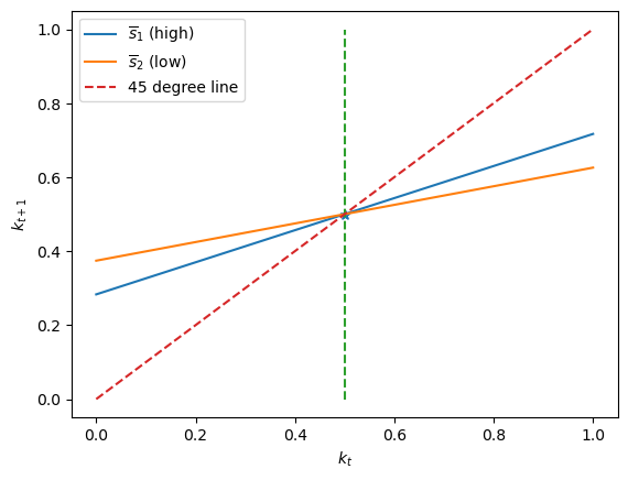
_images/361fde00e13229ed65fd01d8a70391dcd2804d8ddd5f3832edc2ba3014fa66a5.png

The above graph plots $k_{t + 1} = k_{t} + u_{t} = k_{t} - F x_{t}$ as an affine (i.e., linear in $k_{t}$ plus a constant) function of $k_{t}$ for both Markov states $s_{t}$ .

It also plots the 45 degree line.

Notice that the two $s_{t}$ -dependent closed loop functions that determine $k_{t + 1}$ as functions of $k_{t}$ share the same rest point (also called a fixed point) at $k_{t} = 0.5$ .

Evidently, the optimal decision rule in Markov state $2$ , in which the adjustment cost is lower, makes $k_{t + 1}$ a flatter function of $k_{t}$ in Markov state $2$ .

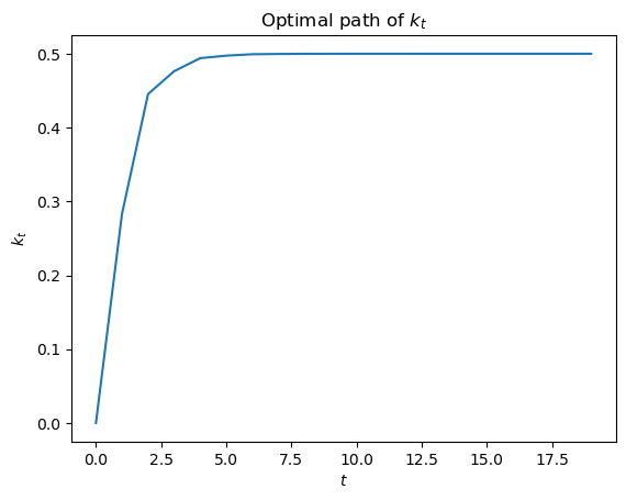
This happens because when $k_{t}$ is not at its fixed point, $| u_{t, 2} | > | u_{t, 2} |$ , so that the decision-maker adjusts toward the fixed point faster when the Markov state $s_{t}$ takes a value that makes it cheaper.

# Compute time series
T = 20
x0 = np.array([[0., 1.]]).T
x_path = ex1_a.compute_sequence(x0, ts_length=T)[0]

fig, ax = plt.subplots()
ax.plot(range(T), x_path[0, :-1])
ax.set_xlabel("$t$")
ax.set_ylabel("$k_t$")
ax.set_title("Optimal path of $k_t$")
plt.show()

_images/dcd86c9f0abf7f2796c3e3ce84ce04dfefcfbb92b133518c1a7aa12f0968dc39.png

Now we’ll depart from the preceding transition matrix that made the Markov state be strictly periodic.

We’ll begin with symmetric transition matrices of the form

\begin{array}{r} Π_{2} = [\begin{array}{c} 1 - λ & λ \\ λ & 1 - λ \end{array}] . \end{array}

λ = 0.8 # high λ
Π2 = np.array([[1-λ, λ],
               [λ, 1-λ]])

ex1_b = qe.LQMarkov(Π2, Qs, Rs, As, Bs, Cs=Cs, Ns=Ns, beta=β)
ex1_b.stationary_values();
ex1_b.Fs

array([[[ 0.57291724, -0.28645862]],

       [[ 0.74434525, -0.37217263]]])

λ = 0.2 # low λ
Π2 = np.array([[1-λ, λ],
               [λ, 1-λ]])

ex1_b = qe.LQMarkov(Π2, Qs, Rs, As, Bs, Cs=Cs, Ns=Ns, beta=β)
ex1_b.stationary_values();
ex1_b.Fs

array([[[ 0.59533259, -0.2976663 ]],

       [[ 0.72818728, -0.36409364]]])

We can plot optimal decision rules associated with different $λ$ values.

λ_vals = np.linspace(0., 1., 10)
F1 = np.empty((λ_vals.size, 2))
F2 = np.empty((λ_vals.size, 2))

for i, λ in enumerate(λ_vals):
    Π2 = np.array([[1-λ, λ],
                   [λ, 1-λ]])

    ex1_b = qe.LQMarkov(Π2, Qs, Rs, As, Bs, Cs=Cs, Ns=Ns, beta=β)
    ex1_b.stationary_values();
    F1[i, :] = ex1_b.Fs[0, 0, :]
    F2[i, :] = ex1_b.Fs[1, 0, :]

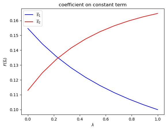
for i, state_var in enumerate(state_vec1):
    fig, ax = plt.subplots()
    ax.plot(λ_vals, F1[:, i], label=r"$\overline{s}_1$", color="b")
    ax.plot(λ_vals, F2[:, i], label=r"$\overline{s}_2$", color="r")

    ax.set_xlabel(r"$\lambda$")
    ax.set_ylabel("$F_{s_t}$")
    ax.set_title(f"Coefficient on {state_var}")
    ax.legend()
    plt.show()

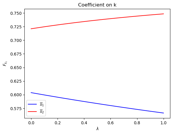
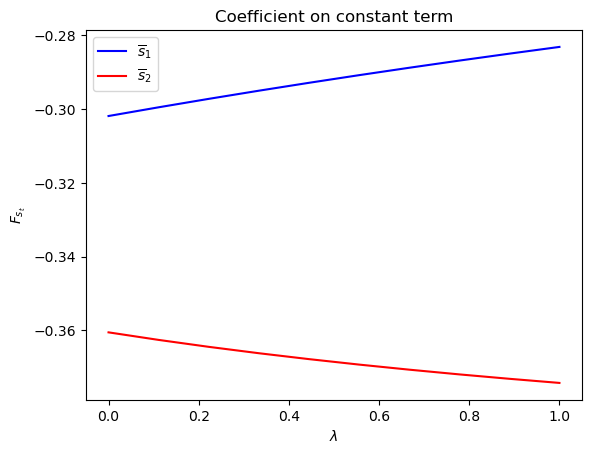
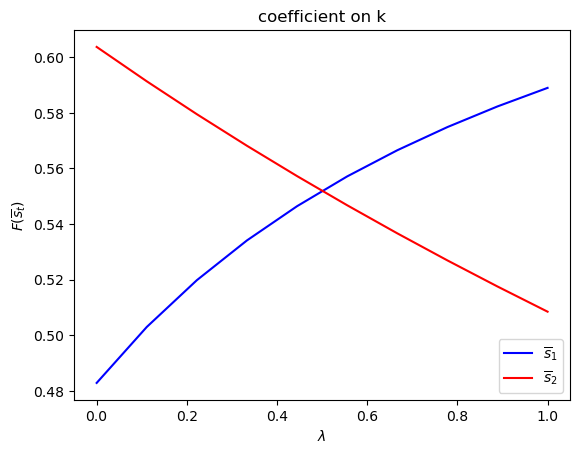
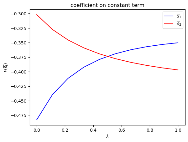
_images/134d58e5bb9a5d4e1a501f0b0e9104df807eb9232bf73275f91ee53a199a0da3.png

_images/17fe63c322edb97e4678b7500109320bc7d33c667bd3e9f546f3e531925dd653.png

Notice how the decision rules’ constants and slopes behave as functions of $λ$ .

Evidently, as the Markov chain becomes more nearly periodic (i.e., as $λ \to 1$ ), the dynamic program adjusts capital faster in the low adjustment cost Markov state to take advantage of what is only temporarily a more favorable time to invest.

Now let’s study situations in which the Markov transition matrix $Π$ is asymmetric

\begin{array}{r} Π_{3} = [\begin{array}{c} 1 - λ & λ \\ δ & 1 - δ \end{array}] . \end{array}

λ, δ = 0.8, 0.2
Π3 = np.array([[1-λ, λ],
               [δ, 1-δ]])

ex1_b = qe.LQMarkov(Π3, Qs, Rs, As, Bs, Cs=Cs, Ns=Ns, beta=β)
ex1_b.stationary_values();
ex1_b.Fs

array([[[ 0.57169781, -0.2858489 ]],

       [[ 0.72749075, -0.36374537]]])

We can plot optimal decision rules for different $λ$ and $δ$ values.

λ_vals = np.linspace(0., 1., 10)
δ_vals = np.linspace(0., 1., 10)

λ_grid = np.empty((λ_vals.size, δ_vals.size))
δ_grid = np.empty((λ_vals.size, δ_vals.size))
F1_grid = np.empty((λ_vals.size, δ_vals.size, len(state_vec1)))
F2_grid = np.empty((λ_vals.size, δ_vals.size, len(state_vec1)))

for i, λ in enumerate(λ_vals):
    λ_grid[i, :] = λ
    δ_grid[i, :] = δ_vals
    for j, δ in enumerate(δ_vals):
        Π3 = np.array([[1-λ, λ],
                       [δ, 1-δ]])

        ex1_b = qe.LQMarkov(Π3, Qs, Rs, As, Bs, Cs=Cs, Ns=Ns, beta=β)
        ex1_b.stationary_values();
        F1_grid[i, j, :] = ex1_b.Fs[0, 0, :]
        F2_grid[i, j, :] = ex1_b.Fs[1, 0, :]

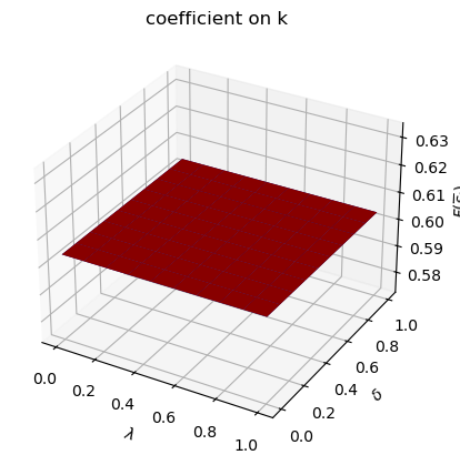
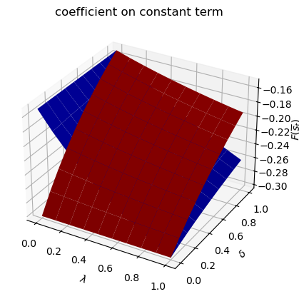
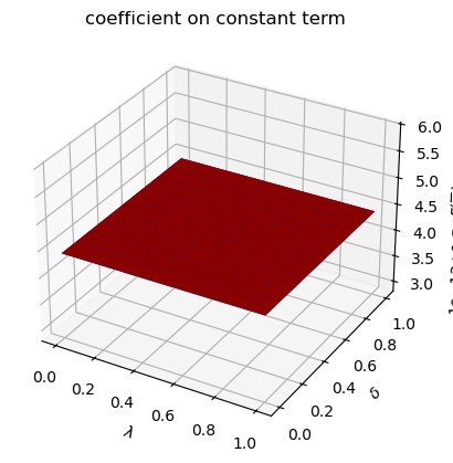
for i, state_var in enumerate(state_vec1):
    fig = plt.figure()
    ax = fig.add_subplot(111, projection='3d')
    # high adjustment cost, blue surface
    ax.plot_surface(λ_grid, δ_grid, F1_grid[:, :, i], color="b")
    # low adjustment cost, red surface
    ax.plot_surface(λ_grid, δ_grid, F2_grid[:, :, i], color="r")
    ax.set_xlabel(r"$\lambda$")
    ax.set_ylabel(r"$\delta$")
    ax.set_zlabel("$F_{s_t}$")
    ax.set_title(f"coefficient on {state_var}")
    plt.show()

_images/6283cc4a9ca060dfd811bf113d5ac3ab8f42321239197c842fd9f5ac2eaa9578.png

_images/f62a64f689b13d1772f094d1f87edb4d4be70bad77bc89a933427bb267a1e4bc.png

The following code defines a wrapper function that computes optimal decision rules for cases with different Markov transition matrices

def run(construct_func, vals_dict, state_vec):
    """
    A Wrapper function that repeats the computation above
    for different cases
    """

    Qs, Rs, Ns, As, Bs, Cs, k_star = construct_func(**vals_dict)

    # Symmetric Π
    # Notice that pure periodic transition is a special case
    # when λ=1
    print("symmetric Π case:\n")
    λ_vals = np.linspace(0., 1., 10)
    F1 = np.empty((λ_vals.size, len(state_vec)))
    F2 = np.empty((λ_vals.size, len(state_vec)))

    for i, λ in enumerate(λ_vals):
        Π2 = np.array([[1-λ, λ],
                       [λ, 1-λ]])

        mplq = qe.LQMarkov(Π2, Qs, Rs, As, Bs, Cs=Cs, Ns=Ns, beta=β)
        mplq.stationary_values();
        F1[i, :] = mplq.Fs[0, 0, :]
        F2[i, :] = mplq.Fs[1, 0, :]

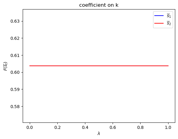
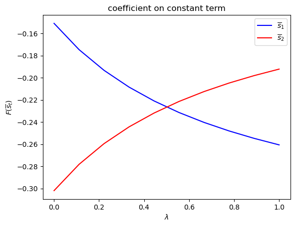
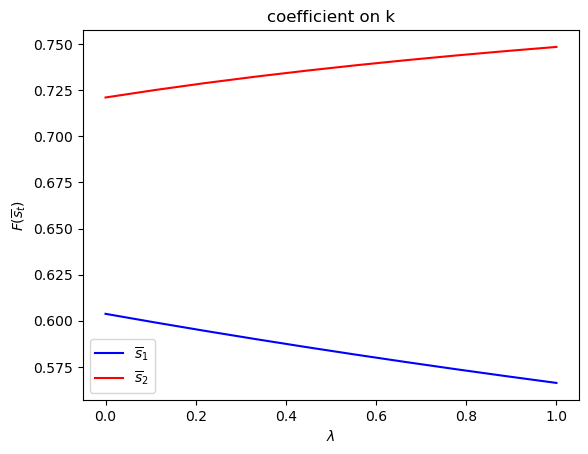
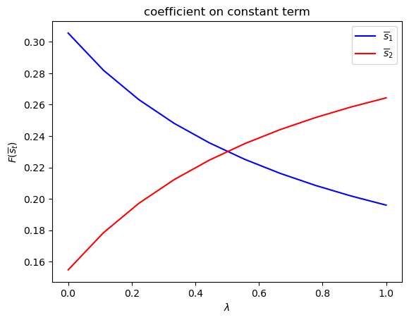
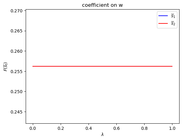
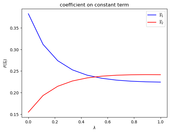
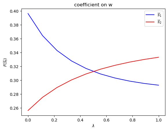
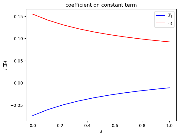
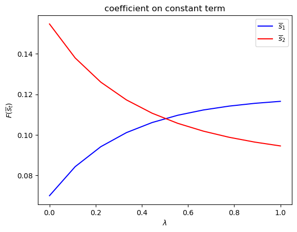
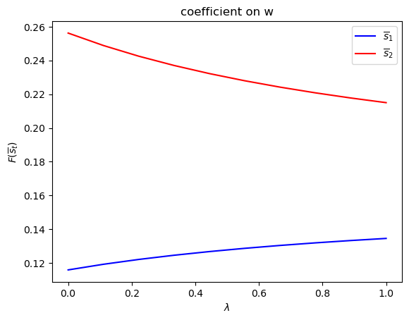
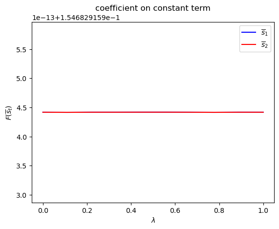
    for i, state_var in enumerate(state_vec):
        fig = plt.figure()
        ax = fig.add_subplot(111)
        ax.plot(λ_vals, F1[:, i], label=r"$\overline{s}_1$", color="b")
        ax.plot(λ_vals, F2[:, i], label=r"$\overline{s}_2$", color="r")

        ax.set_xlabel(r"$\lambda$")
        ax.set_ylabel(r"$F(\overline{s}_t)$")
        ax.set_title(f"coefficient on {state_var}")
        ax.legend()
        plt.show()

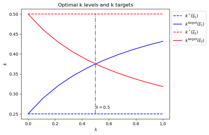
    # Plot optimal k*_{s_t} and k that optimal policies are targeting
    # only for example 1
    if state_vec == ["k", "constant term"]:
        fig = plt.figure()
        ax = fig.add_subplot(111)
        for i in range(2):
            F = [F1, F2][i]
            c = ["b", "r"][i]
            ax.plot([0, 1], [k_star[i], k_star[i]], "--",
                    color=c, label=r"$k^*(\overline{s}_"+str(i+1)+")$")
            ax.plot(λ_vals, - F[:, 1] / F[:, 0], color=c,
                    label=r"$k^{target}(\overline{s}_"+str(i+1)+")$")

        # Plot a vertical line at λ=0.5
        ax.plot([0.5, 0.5], [min(k_star), max(k_star)], "-.")

        ax.set_xlabel(r"$\lambda$")
        ax.set_ylabel("$k$")
        ax.set_title("Optimal k levels and k targets")
        ax.text(0.5, min(k_star)+(max(k_star)-min(k_star))/20, r"$\lambda=0.5$")
        ax.legend(bbox_to_anchor=(1., 1.))
        plt.show()

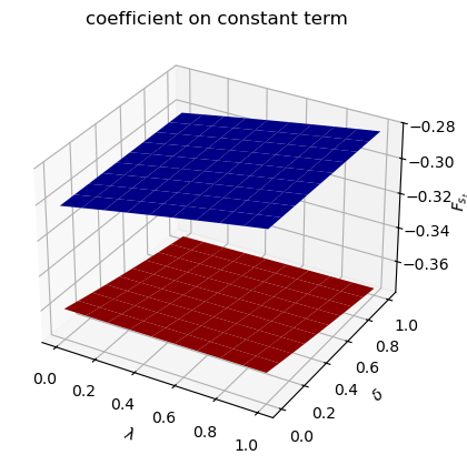
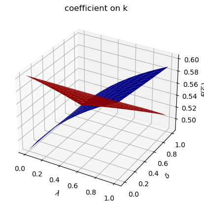
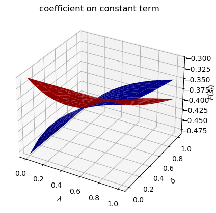
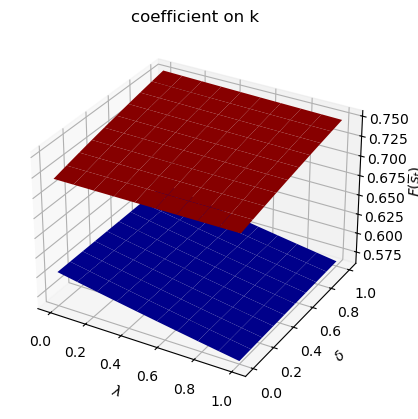
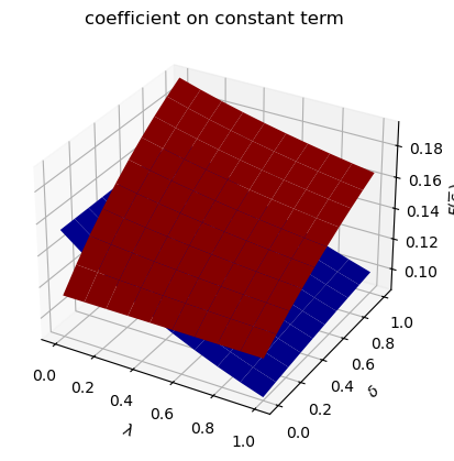
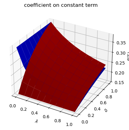
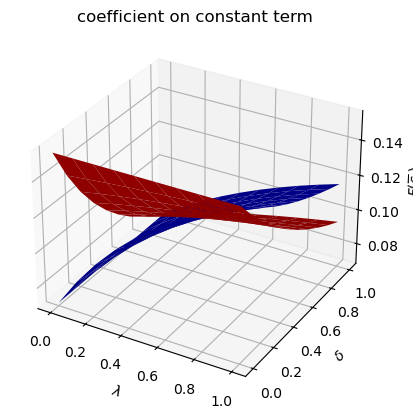
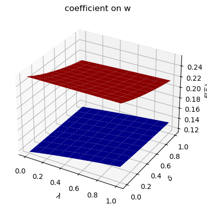
    # Asymmetric Π
    print("asymmetric Π case:\n")
    δ_vals = np.linspace(0., 1., 10)

    λ_grid = np.empty((λ_vals.size, δ_vals.size))
    δ_grid = np.empty((λ_vals.size, δ_vals.size))
    F1_grid = np.empty((λ_vals.size, δ_vals.size, len(state_vec)))
    F2_grid = np.empty((λ_vals.size, δ_vals.size, len(state_vec)))

    for i, λ in enumerate(λ_vals):
        λ_grid[i, :] = λ
        δ_grid[i, :] = δ_vals
        for j, δ in enumerate(δ_vals):
            Π3 = np.array([[1-λ, λ],
                           [δ, 1-δ]])

            mplq = qe.LQMarkov(Π3, Qs, Rs, As, Bs, Cs=Cs, Ns=Ns, beta=β)
            mplq.stationary_values();
            F1_grid[i, j, :] = mplq.Fs[0, 0, :]
            F2_grid[i, j, :] = mplq.Fs[1, 0, :]

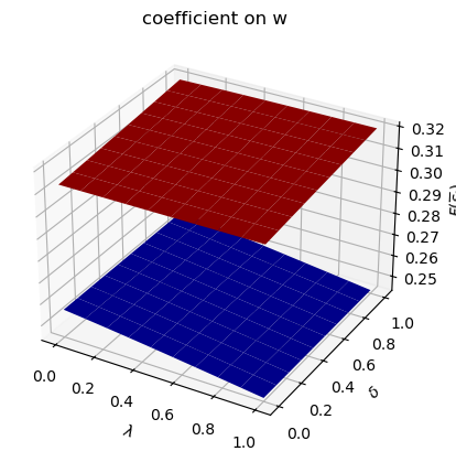
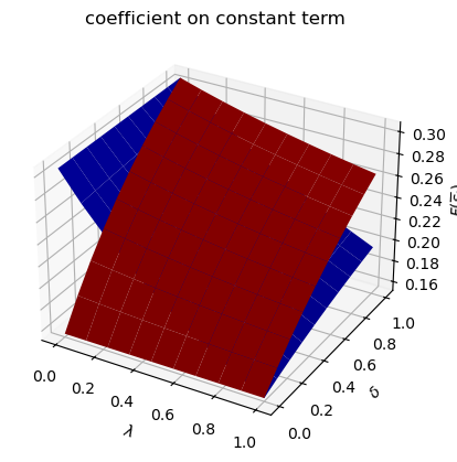
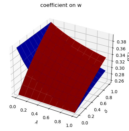
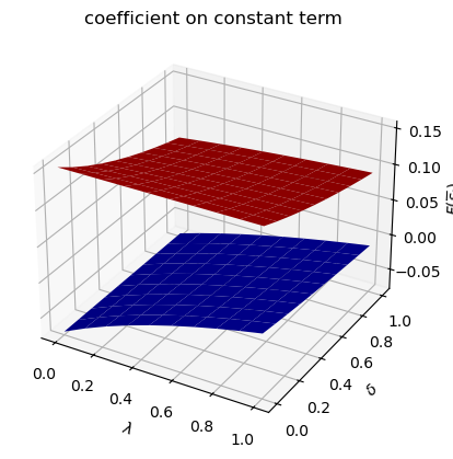
    for i, state_var in enumerate(state_vec):
        fig = plt.figure()
        ax = fig.add_subplot(111, projection='3d')
        ax.plot_surface(λ_grid, δ_grid, F1_grid[:, :, i], color="b")
        ax.plot_surface(λ_grid, δ_grid, F2_grid[:, :, i], color="r")
        ax.set_xlabel(r"$\lambda$")
        ax.set_ylabel(r"$\delta$")
        ax.set_zlabel(r"$F(\overline{s}_t)$")
        ax.set_title(f"coefficient on {state_var}")
        plt.show()

To illustrate the code with another example, we shall set $f_{2, s_{t}}$ and $d_{s_{t}}$ as constant functions and

f_{1, 1} = 0.5, f_{1, 2} = 1

Thus, the sole role of the Markov jump state $s_{t}$ is to identify times in which capital is very productive and other times in which it is less productive.

The example below reveals much about the structure of the optimum problem and optimal policies.

Only $f_{1, s_{t}}$ varies with $s_{t}$ .

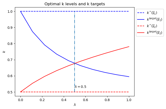
So there are different $s_{t}$ -dependent optimal static $k$ level in different states $k_{s_{t}}^{*} = \frac{f_{1, s_{t}}}{2 f_{2, s_{t}}}$ , values of $k$ that maximize one-period payoff functions in each state.

We denote a target $k$ level as $k_{s_{t}}^{t a r g e t}$ , the fixed point of the optimal policies in each state, given the value of $λ$ .

We call $k_{s_{t}}^{t a r g e t}$ a “target” because in each Markov state $s_{t}$ , optimal policies are contraction mappings and will push $k_{t}$ towards a fixed point $k_{s_{t}}^{t a r g e t}$ .

When $λ \to 0$ , each Markov state becomes close to absorbing state and consequently $k_{s_{t}}^{t a r g e t} \to k_{s_{t}}^{*}$ .

But when $λ \to 1$ , the Markov transition matrix becomes more nearly periodic, so the optimum decision rules target more at the optimal $k$ level in the other state in order to enjoy higher expected payoff in the next period.

The switch happens at $λ = 0.5$ when both states are equally likely to be reached.

Below we plot an additional figure that shows optimal $k$ levels in the two states Markov jump state and also how the targeted $k$ levels change as $λ$ changes.

run(construct_arrays1, {"f1_vals":[0.5, 1.]}, state_vec1)

symmetric Π case:

_images/b27302ccbfbd9b3c2c30dca0197c9ef373e4132914480c1628dbeab9070fc649.png

_images/4dc9976641fdc3614660167aee20db748d554ada34e314bdd6d3a85645db48b6.png

_images/d1446a9d7118e84152a00f3cd3666555ee2453229063ebd9ae9805933ae87a7a.png

asymmetric Π case:

_images/a6c194e104f2199ea87c336a5830633b2052f466fd291411c255aa27f0df3064.png

_images/aad447205db80b20a3c91201fc96f405b17972cfa0add1dbdd842120ac2648d3.png

Set $f_{1, s_{t}}$ and $d_{s_{t}}$ as constant functions and

f_{2, 1} = 0.5, f_{2, 2} = 1

run(construct_arrays1, {"f2_vals":[0.5, 1.]}, state_vec1)

symmetric Π case:

_images/dba8506d886eebdbaca2804f9a27d3d282bf21f1f2edcdbf4d0ce56caeb59f65.png

_images/87d9218fbc30cf597d81fd8669c63d9ce504a521bf18810dca6472211fff683d.png

_images/ce43701af54f120543485a5df76b27e5fef60713ce711e28279031856f949083.png

asymmetric Π case:

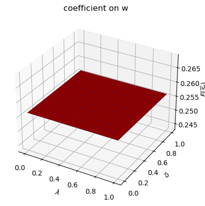
_images/97618bf0b5d4fdc60d634572ae50ce7946e664bdb2da50245e01ec13c82f534e.png

_images/f3ba1df1aba60178b316ff5a3c26c953c85a1a33c3f7120a12ea0d0e0e8ff0c8.png

8.6. Example 2#

We now add to the example 1 setup another state variable $w_{t}$ that follows the evolution law

w_{t + 1} = α_{0} (s_{t}) + ρ (s_{t}) w_{t} + σ (s_{t}) ε_{t + 1}, ε_{t + 1} \sim N (0, 1)

We think of $w_{t}$ as a rental rate or tax rate that the decision maker pays each period for $k_{t}$ .

To capture this idea, we add to the decision-maker’s one-period payoff function the product of $w_{t}$ and $k_{t}$

r (s_{t}, k_{t}, w_{t}) = f_{1, s_{t}} k_{t} - f_{2, s_{t}} k_{t}^{2} - d_{s_{t}} (k_{t + 1} - k_{t})^{2} - w_{t} k_{t},

We now let the continuous part of the state at time $t$ be $x_{t} = [\begin{matrix} k_{t} \\ 1 \\ w_{t} \end{matrix}]$ and continue to set the control $u_{t} = k_{t + 1} - k_{t}$ .

We can write the one-period payoff function $r (s_{t}, k_{t}, w_{t})$ as

\begin{array}{r} \begin{aligned} r (s_{t}, k_{t}, w_{t}) & = f_{1} (s_{t}) k_{t} - f_{2} (s_{t}) k_{t}^{2} - d (s_{t}) {(k_{t + 1} - k_{t})}^{2} - w_{t} k_{t} \\ = - (x_{t}^{'} \underset{\equiv R (s_{t})}{\underset{⏟}{[\begin{array}{c} f_{2} (s_{t}) & - \frac{f_{1} (s_{t})}{2} & \frac{1}{2} \\ - \frac{f_{1} (s_{t})}{2} & 0 & 0 \\ \frac{1}{2} & 0 & 0 \end{array}]}} x_{t} + \underset{\equiv Q (s_{t})}{\underset{⏟}{d (s_{t})}} u_{t}^{2}), \end{aligned} \end{array}

and the state-transition law as

\begin{array}{r} x_{t + 1} = [\begin{array}{c} k_{t + 1} \\ 1 \\ w_{t + 1} \end{array}] = \underset{\equiv A (s_{t})}{\underset{⏟}{[\begin{array}{c} 1 & 0 & 0 \\ 0 & 1 & 0 \\ 0 & α_{0} (s_{t}) & ρ (s_{t}) \end{array}]}} x_{t} + \underset{\equiv B (s_{t})}{\underset{⏟}{[\begin{array}{c} 1 \\ 0 \\ 0 \end{array}]}} u_{t} + \underset{\equiv C (s_{t})}{\underset{⏟}{[\begin{array}{c} 0 \\ 0 \\ σ (s_{t}) \end{array}]}} ε_{t + 1} \end{array}

def construct_arrays2(f1_vals=[1. ,1.],
                      f2_vals=[1., 1.],
                      d_vals=[1., 1.],
                      α0_vals=[1., 1.],
                      ρ_vals=[0.9, 0.9],
                      σ_vals=[1., 1.]):
    """
    Construct matrices that maps the problem described in example 2
    into a Markov jump linear quadratic dynamic programming problem.
    """

    m = len(f1_vals)
    n, k, j = 3, 1, 1

    Rs = np.zeros((m, n, n))
    Qs = np.zeros((m, k, k))
    As = np.zeros((m, n, n))
    Bs = np.zeros((m, n, k))
    Cs = np.zeros((m, n, j))

    for i in range(m):
        Rs[i, 0, 0] = f2_vals[i]
        Rs[i, 1, 0] = - f1_vals[i] / 2
        Rs[i, 0, 1] = - f1_vals[i] / 2
        Rs[i, 0, 2] = 1/2
        Rs[i, 2, 0] = 1/2

        Qs[i, 0, 0] = d_vals[i]

        As[i, 0, 0] = 1
        As[i, 1, 1] = 1
        As[i, 2, 1] = α0_vals[i]
        As[i, 2, 2] = ρ_vals[i]

        Bs[i, :, :] = np.array([[1, 0, 0]]).T

        Cs[i, :, :] = np.array([[0, 0, σ_vals[i]]]).T

    Ns = None
    k_star = None

    return Qs, Rs, Ns, As, Bs, Cs, k_star

state_vec2 = ["k", "constant term", "w"]

Only $d_{s_{t}}$ depends on $s_{t}$ .

run(construct_arrays2, {"d_vals":[1., 0.5]}, state_vec2)

symmetric Π case:

_images/b38c41a68b4f2b7efaefa351e65d62b28c6b64eafdeb07a75c030003951e6255.png

_images/263fd36b53910623f3763145aabea5b09e3d78e22f25b208762b7ed1baab01a8.png

_images/34fc0d00e00900c41966112a73bc68c4fb89946c5fd8c9b4673f6df31296da04.png

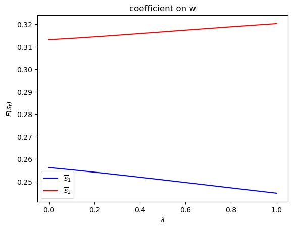
asymmetric Π case:

_images/fd2be1a2249a3baf1e1925a2618eb8a3f0b18a18a685a61f132d06269991d033.png

_images/e2e74516253d6245967ebf28899238cbb7882e7a3b005a83eb6ea67d248d6fea.png

_images/be8fa9b038e287a8e46c7e3078da5dae0558ad0cb6b7ea32ea8a8fa8672d67b2.png

Only $f_{1, s_{t}}$ depends on $s_{t}$ .

run(construct_arrays2, {"f1_vals":[0.5, 1.]}, state_vec2)

symmetric Π case:

_images/6623b698ed7c60f6a7e833061a2a8c574f22d44fca5cc88e3f7f5d18d339d870.png

_images/436330f23fee2249430c94612fcc4a0959e66c6fa0d35b8f58a8d836fdbbc9b4.png

asymmetric Π case:

_images/96a08070383d7c23d8e6a5adebe053ea540e3eecc016a8909133e36b14d350d0.png

_images/70576603fb07f750502e72a867e8f22e6c71dde816f33d89a3e0fcbdf1642329.png

Only $f_{2, s_{t}}$ depends on $s_{t}$ .

run(construct_arrays2, {"f2_vals":[0.5, 1.]}, state_vec2)

symmetric Π case:

_images/61b6b3243edb2f66e4b1b1db73ada2dc650b2ab36ac298e89cd53ef3aef21f27.png

_images/418f2f210ea81a63ee2d6d08f8b2137808060141177cc197cb3fb223f690e561.png

asymmetric Π case:

_images/28413c4e3cf2f88e5442d773720bef5b7f884d4c8dc7fee4d5a56eb72133a23e.png

_images/008932b152e723a7bf41575f5f980f7ef4f70c9475211237a170ed6229fd9738.png

Only $α_{0} (s_{t})$ depends on $s_{t}$ .

run(construct_arrays2, {"α0_vals":[0.5, 1.]}, state_vec2)

symmetric Π case:

_images/cb118b38b366ff4453aa0a5aabca56c8d7fad1dac3dbec307758ad9dbed810b6.png

asymmetric Π case:

_images/22c8e6ae0b4728127582e6f9e67b1974031cb057ed7a0c88c3d0a0559c3e9d0c.png

Only $ρ_{s_{t}}$ depends on $s_{t}$ .

run(construct_arrays2, {"ρ_vals":[0.5, 0.9]}, state_vec2)

symmetric Π case:

_images/66c1951774d2b4a806cb21091b982e66319c919772d366cf2cb6e2de136eba85.png

_images/6e69423146ebd7990c38a41c6fa048a1a1613ef7f8ce0947bceea83ef0a6750d.png

asymmetric Π case:

_images/61031f2ca7e4e08d9745c6fe5f439536f9de7319033fb024b12b65901f84370b.png

_images/ce8d8f11aa089ce7178f768b4a5cfd0bcc6e3d8bde0d61f65645085ab4c061f1.png

Only $σ_{s_{t}}$ depends on $s_{t}$ .

run(construct_arrays2, {"σ_vals":[0.5, 1.]}, state_vec2)

symmetric Π case:

_images/e684721b6068f43b2a5afa2f8065460074662cb87ac17b70e2a760bb379e02c7.png

asymmetric Π case:

_images/78b4a4c28ccab10679a0a734a20cdbdc3d3a9c84663120b8ba5ddc6b137dc12e.png

8.7. More examples#

The following lectures describe how Markov jump linear quadratic dynamic programming can be used to extend the [Barro, 1979] model of optimal tax-smoothing and government debt in several interesting directions